Sensor Data Fusion Using a Probability Density Grid - ISIF

Sensor Data Fusion Using a Probability Density Grid
Derek Elsaesser
Communication and Navigation Electronic Warfare Section
DRDC Ottawa
Defence R&D Canada
Derek.Elsaesser@drdc-rddc.gc.ca
Abstract - A novel technique has been developed at
DRDC Ottawa for fusing Electronic Warfare (EW)
sensor data by numerically combining the probability
density function representing the measured value and
error estimate provided by each sensor. Multiple
measurements are sampled at common discrete intervals
to form a probability density grid and combined to
produce the fused estimate of the measured parameter.
This technique, called the Discrete Probability Density
(DPD) method, is used to combine sensor measurements
taken from different locations for the EW function of
emitter geolocation. Results are presented using
simulated line of bearing measurements and are shown
to approach the theoretical location accuracy limit
predicted by the Cramer-Rao Lower Bound. The DPD
method is proposed for fusing other geolocation sensor
data including time of arrival, time difference of arrival,
and a priori information.
Keywords: Sensor data fusion, discrete probability
density, emitter location estimation.
1 Introduction
The Discrete Probability Density (DPD) method is a novel
technique developed at Defence R&D Canada for
numerically combining data containing uncertainty, such
as Electronic Warfare (EW) sensor measurements [1, 2, 3,
4, 5]. The basic assumption is that the sensor
measurement of a given parameter can be modeled by
some probability density function (PDF) over the range of
possible values. The PDF may be modeled by a function,
such as a Gaussian distribution, or by a set of empirical
values that reflect the probability of the true value
occurring within some range of the measured value.
The basic theory of the DPD method is presented in
Section 2. It describes the process for sampling
independent PDFs at common discrete intervals to
produce a set of discrete probability density vectors which
are combined to form a joint DPD vector for estimating
the mean and variance of the fused estimate of the
measured parameter. Section 3 describes how this method
is used to combine data from multiple sensor locations by
projecting measurements of a common parameter onto a
two-dimensional probability density grid. This is used to
determine the most likely coordinates of the object being
measured and an error estimate.
In section 4 the DPD method is applied to emitter
geolocation using line of bearing (LOB) measurements
from multiple sensor locations [3]. The performance of
the DPD method for emitter location accuracy is
compared to the theoretical Cramer-Rao Lower Bound
(CRLB) [6] as a function of the number of measurements
included. The use of the DPD to fuse other sensor data,
such as time of arrival (TOA), time difference of arrival
(TDOA), and a priori information, is presented in section
5.
2 Discrete Probability Density Theory
Data with uncertainty, such as sensor measurements, can
be modeled by some PDF over the range of possible
values. These PDFs may be represented by various
distributions. Unlike techniques that use systems of
equations to combine multiple sensor measurements and
minimize the resulting error estimate, the DPD method
combines probability density distributions of
measurements directly by sampling each PDF at common
intervals and calculating the joint product over the sample
space. The resulting discrete probability density
distribution is then used to calculate the estimated value
and variance of the measured parameter. This concept is
introduced using a one-dimensional DPD vector.
2.1 Discrete Sampling of Probability
Density Functions
All inputs are assumed to be estimates of some parameter,
x, expressed as a probability density function, f X (x),
representing the uncertainty or error in the estimated value
of x [7]. The discrete probability density vector is formed
by evaluating f X (x) at discrete points over the range of
possible values of x. Let X(n) represent the discrete values
of x over the range [a, b] sampled at intervals of ∆x with
a delta function δ(n):
b
X ( n)
= xδ ( x − ∆x n)
n = 1…
N (1)
x = a
The DPD vector is formed by evaluating the PDF at each
value of X(n), with the integer indices of the DPD vector,
n, then representing discrete values of x:
F ( n)
= f ( X ( n))
n = 1…
N
(2)
x
x

This requires the total area under f X (x) equals unity and the
value of f X (x) > 0 over the range of possible values of x. If
the value of the PDF is zero over some range of x, it
implies that it is impossible for the measured value of x to
occur in this range. As the DPD vector is produced by
discrete sampling of a PDF, the DPD method is not reliant
on a specific probability distribution and can be used with
a variety of probability density distributions, including
non-linear distributions.
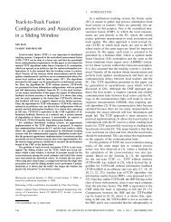
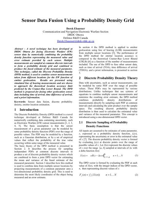
As an example of a DPD vector, consider the Gaussian
PDF which is commonly used to represent sensor
measurement errors that are normally distributed. It can be
described by a mean, representing the estimated value,
and variance, representing the uncertainty [4]. It can also
be used in a system of equations representing the
combination of multiple measurements for applications
such as geolocation. A sensor measurement produces an
estimate of x = 20 with a standard deviation of σ = 9.0.
The Gaussian PDF is sampled over the range [-10, 50] at
intervals of ∆x = 3.0. The continuous Gaussian PDF and
the resulting DPD vector are shown in Figure 1. They are
normalized over the range of x and the index, n, of F X (n)
is translated back into x for comparison with f X (x).
f(x), F(x)
Continuous and Discrete Gaussian pdf; mean = 20.0, std = 9.0, dx = 3.0
0.05
continuous pdf
0.045
discrete pdf
0.04
0.035
0.03
0.025
0.02
0.015
0.01
0.005
0
-7 -4 -1 2 5 8 11 14 17 20 23 26 29 32 35 38 41 44 47 50
x
Figure 1. Discrete sampling of a Gaussian PDF
2.2 Selecting a Sampling Interval
Selection of an appropriate sampling interval, ∆x, is
important as it directly impacts the computational cost of
combining multiple measurements. In order to minimize
the number of points, N, sampled over the range of x, the
sampling interval must be selected so that the nature of the
distribution of f X (x) is maintained by F X (n). As the aim is
to determine the estimated value of x, x , and an error
estimate in the form of the variance, σ 2 , about x , the
sampling interval can be relatively large with respect to
the variation in f X (x). For combining a set of Gaussian
PDFs, a sampling interval of approximately σ i /2 (using the
smallest value of σ i from the PDFs) has been found to be
sufficient. Sampling at smaller intervals is generally found
to have little effect on the resulting value of x and σ 2 , but
increases computational cost proportionately with number
of samples. Another factor to consider is the desired
resolution of the resulting estimate of x . Because the
index, n, of F X (n) is used to determine x , the sampling
interval should be smaller than the desired resolution in x.
2.3 Joint DPD Vectors
A joint DPD vector is formed by taking the product of
each input PDF at common sample points, X(n). For S
sensor measurements this is expressed as:
F ( s,
n)
= f ( s,
X ( n))
n = 1…
N (3)
x
x
where s = 1…S independent measurements of the same
target; f X (s, x) is the array of PDFs representing these
measurements over the same range [a, b] of x; and F X (s, n)
is the resulting array of DPD vectors of length N. The
joint discrete probability density vector, P X (n), is
determined by taking the product of all DPD vectors at
each integer value of n:
S
'
PX
( n)
= ∏ FX
( s,
n)
n = 1…
N (4)
s=
1
then calculating the normalization constant C:
C =
N
∑
n=
1
'
P X
( n)
(5)
resulting in the joint DPD vector:
1 '
PX
( n)
= PX
( n)
C
n = 1…
N (6)
It is assumed that the chosen sampling interval is small
enough to realize the significant variations in P X (n).
The estimated value of the fused result is determined from
the indices n weighted by P X (n):
N
n = ∑
n=
1
nP n X
( )
and the estimated variance of n by:
∑
n=
1
(7)
N
2 2
σ = ( n − n)
P ( n)
(8)
n
This is translated back into the domain of X within the
range [a, b] giving the estimated value of x as:
x = ∆xn
+ a
The standard deviation representing the combined error
estimate is given by:
σ = ∆
(10)
X
xσ n
X
(9)

As the estimated value and error of the combined
measurements, x andσ
X
, are produced by evaluating
each PDF at discrete points, the DPD method can be used
to combine measurements with different types of
probability density distributions.
2.4 Combining Sensor Measurements
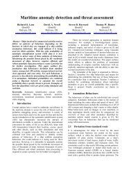
Benefits of the DPD method can be demonstrated by the
following example, where the target value, x T =30, and
each sensor measurement is modeled as a Gaussian PDF,
PDF i (µ,σ), i = 1…3, with the mean being the measured
value and the error estimate being the standard deviation.
Note that each f X (x) must always be greater than 0. It is
assumed that PDF 1 and PDF 3 represent accurate,
unbiased, measurements of x T , but PDF 2 is a ‘wild’ or
biased estimate. These three PDFs are shown in Figure 2,
sampled at interval ∆x = 1.5 in Figure 3. The values of
x and σ are calculated from the joint DPD vector shown
X
in Figure 4. It is seen that the inclusion of the biased
measurement has only a modest effect on the resulting
estimated value, x = 29.7, and error estimate, σ = 3.7.
Gaussian(mean, std) for PDF1(30.0, 3.0), PDF2(11.5, 4.0), PDF3(30.5, 5.0)
0.14
PDF1
PDF2
0.12
PDF3
f(x)
F(x)
0.1
0.08
0.06
0.04
0.02
0
0 10 20 30 40 50 60
x
Figure 2. Three sensor measurements of x T = 30
0.14
0.12
0.1
0.08
0.06
0.04
0.02
0
Discrete Sampling of Multiple PDFs, dx = 1.5
6 12 18 24 30 36 42 48 54 60
x
X
PDF1
PDF2
PDF3
Figure 3. Discrete sampling of measurement PDFs
P(x)
0.25
0.2
0.15
0.1
0.05
0
Discrete Joint DPD, E[x] = 29.7, STD[x] = 3.7, dx = 1.5
6 12 18 24 30 36 42 48 54 60
x
Figure 4. Joint DPD vector estimate of x T
Numerous Monte Carlo simulations were conducted using
combinations of various standard deviations, bias errors,
and large numbers of measurements [2]. It was found that
the joint DPD estimate generally converged on the true
value as the number of measurements increased. It was
also seen that the estimate was resilient to inclusion of
measurements with large bias errors, with the main effect
being an increase in the magnitude of the error estimate.
3 Two Dimensional DPD Grids
A common data fusion function is to combine sensor
measurements from multiple reference points to determine
an estimate of the target in two or more dimensions. An
example is emitter geolocation using LOB or TDOA
measurements from multiple sensor positions [3]. The
DPD method is applied by projecting the measurement
PDF from each sensor onto a common grid of sample
points. This requires that some transform function exists
that will map the measured parameter into 2-dimenional
space. This section describes using bearing measurements
to produce a 2-dimensional location estimate.
3.1 Projecting a LOB into Two Dimensions
The Area-Of-Interest (AOI) that includes the target object
is defined over a region in X and Y using a 2-dimenisonal
grid of points at sample intervals ∆x and ∆y. It is implied
that the target object is located within these bounds. The
AOI must be large enough to ensure that truncation of the
probability distribution at the boundaries does not
significantly affect the result and that the sample interval
is small enough to realize each PDF. Let there be S
independent LOB measurements from sensor positions (x i ,
y i ), i = 1…S, each with a measured bearing µ i and error
estimate σ i . As bearing is an angular measurement, a LOB
measurement can be represented by a von Mises PDF [7]:
f ( θ ) = exp( κ cos( θ − µ )) / 2πI
0
( κ)
0 ≤ θ < 2π
(11)

where θ is the variable in radian, µ is the mean, κ is the
concentration (which is analogous to 1/σ 2 ), and I 0 (κ ) is a
Bessel function of the first kind and order zero. Examples
of the von Mises PDF for LOBs with different values of κ
are shown in Figure 5. Note that other probability density
distributions can be used to model a LOB.
0.16
0.14
Von Mises Probability Density Function
LOB RMS error = 3 degrees, k = 364.7563
LOB RMS error = 6 degrees, k = 91.1891
LOB RMS error = 12 degrees, k = 22.7973
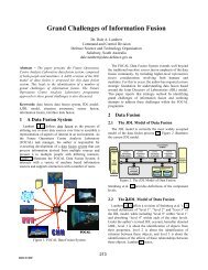
An example of F XY (n,m) for a sensor at position (20, 20)
with bearing estimate µ i = 45° and error estimate σ i = 3° is
shown in Figure 7 as a color surface plot. It is seen that
the value of F(x, y) is constant along any bearing line from
the sensor, regardless of distance, since the value of the
LOB PDF is constant for a given angle.
0.12
0.1
p(angle)
0.08
0.06
0.04
0.02
0
-80 -60 -40 -20 0 20 40 60 80
angle (degrees)
Figure 5. The von Mises PDF used to model a LOB
A transform is required to project the 1-dimensional LOB
measurement, represented as an angular PDF, onto the 2-
dimensional grid in X, Y. The value of the LOB PDF at
each node in the grid is calculated using its angle relative
to the sensor position. The angular transform function
between the sensor location and a grid point is simply [5]:
θ i ( x,
y)
= arctan(( y − y i ) /( x − x i )) − π ≤ θi
< π (12)
The value of a LOB PDF is calculated using the von
Mises PDF with κ = 1/σ 2 for θ i (x, y) – µ i at each discrete
point X(n) and Y(m), representing each (x, y) value in the
grid, as shown in Figure 6.
x i
,y i
x,y
Figure 6. Transforming a LOB PDF to a 2-D DPD grid
This produces a 2-dimensional LOB DPD array:
F XY
( n,
m)
= f ( θ ( X ( n),
Y ( m)))
n = 1... N , m = 1...
M (13)
i
where F XY (n, m) is the LOB DPD array of size N×M
points. The value of F XY (n, m) at a given index is the LOB
PDF, f(θ i ), taken at discrete values of x, y.
θ i
µ i
Figure 7. Example of a 2-D LOB DPD for µ=45˚, σ=3˚
3.2 Joint DPD Location Estimate
For multiple LOB measurements the joint DPD array is
calculated over a common N×M grid by:
S
P
'
XY
( n,
m)
= ∏ FXY
( s,
n,
m)
n = 1... N,
m = 1...
M
s=
1
(14)
where F XY (s, n, m) is the set of S independent LOB DPD
arrays using a common grid. This is normalized by:
N M
C =
'
∑∑P
( n,
m)
(15)
XY
n= 1m=
1
to produce the joint DPD array representing the target
object’s location estimate:
1 '
PXY ( n,
m)
= PXY
( n,
m)
(16)
C
For a grid of N by M points, the resulting computational
complexity of the joint DPD array is of O(S×N×M).
The 2-dimensional location estimate of the target, x T , yT
,
is determined by first taking the Probability Mass
Functions (PMF) of P XY (n, m):
X
M
XY
m=
1
PMF ( n)
= ∑ P ( n,
m)
n = 1... N (17)
N
XY
n=
1
PMF ( m)
= ∑ P ( n,
m)
m = 1... M (18)
Y
The target location estimate can be determined by treating
PMF X (n) and PMF Y (m) as 1-dimensional DPD vectors and

calculating the index estimates, n ˆ , mˆ
T T
, as in equation 7.
For cases where a large number of measurements
correlate, the distribution of P XY (n,m) becomes
exponential about the estimated location. The estimated
location can then be found from the indices that have the
largest values of PMF X (n) and PMF Y (m), respectively. As
the indices are translated back into x and y coordinates to
provide the location estimate of the target, this approach
has the drawback that the resolution of the target location
is limited to the sampling interval.
The location error estimate is determined by the variances
and covariance of the joint DPD array about the indices of
estimated target location:
COV
XY
N
∑
n=
1
2
2
σ = PMF ( n)
⋅ ( n − nˆ
) (19)
X
M
∑
m=
1
X
2
2
σ = PMF ( m)
⋅ ( m − mˆ
) (20)
N
Y
M
= ∑∑
n= 1 m=
1
P
XY
Y
( n,
m)
⋅ ( n − nˆ
) ⋅(
m − mˆ
)
T
T
T
T
(21)
These terms are scaled by the sampling interval and form
a covariance matrix for calculating an Elliptical Error
Probable (EEP), which is commonly used to represent the
error estimate [3]. Although the EEP assumes that the
error distribution is Gaussian, which may not be the case
for a DPD distribution, it is useful for comparing the DPD
results to other geolocation techniques and the CRLB. In
cases where a sufficiently large number of measurements
correlate near a point, the joint DPD distribution is seen to
approximate a Gaussian distribution.
4 DPD Method for LOB Geolocation
LOB data is used for location estimation using the
technique commonly referred to as triangulation. The
DPD method is applied to LOB geolocation and compared
to the CRLB, which represents the performance bound of
an unbiased location estimator for the relative sensor
positions and error estimates, excluding measurement
biases. This is used to assess the accuracy of the DPD
method and its resilience to bias errors.
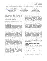
4.1 Increasing the Number of LOBs
The comparison of the DPD method to the CRLB is
conducted using Monte Carlo simulation and averaged
over 10,000 iterations. All LOBs are normally distributed,
with σ = 3˚, from 4 to 10 sensor sites arranged as a linear
baseline across the bottom of an AOI. The details of the
testing are provided in [2]. The AOI is defined as a
200×300 point grid with a sampling interval of 100
meters. The effect on the DPD location estimate is
compared to the CRLB for an increasing number of
unbiased LOBs with LOB1 having a bias error. This is
repeated for bias errors on LOB1 of -40°, -20°, 0, 20°, and
40° counterclockwise. An example for 10 LOBs and a 40°
bias on LOB1 is shown in Figure 8. The location RMSE
for increasing number of LOBs is shown in Figure 9.
Location RMSE (m)
Location RMSE (m)
Location RMSE (m)
Location RMSE (m)
Location RMSE (m)
Y x 100m
300
250
200
150
100
50
Figure 8. Example scenario with LOB1 bias = 40°
4000
2000
LOB STD = 3.0 deg, LOB1 Bias = -40.0 deg
CRLB
DPD Method
0
4 5 6 7 8 9 10
Number of LOBs included in fix
LOB STD = 3.0 deg, LOB1 Bias = -20.0 deg
4000
2000
CRLB
DPD Method
0
4 5 6 7 8 9 10
Number of LOBs included in fix
LOB STD = 3.0 deg, LOB1 Bias = 0.0 deg
4000
2000
CRLB
DPD Method
0
4 5 6 7 8 9 10
Number of LOBs included in fix
LOB STD = 3.0 deg, LOB1 Bias = 20.0 deg
4000
2000
CRLB
DPD Method
0
4 5 6 7 8 9 10
Number of LOBs included in fix
LOB STD = 3.0 deg, LOB1 Bias = 40.0 deg
4000
2000
DPD Location Estimate and CRLB
LOB1
DPD
CRLB
1 5 7 2 9 10 3 8 6 4
20 40 60 80 100 120 140 160 180 200
X x 100m
CRLB
DPD Method
0
4 5 6 7 8 9 10
Number of LOBs included in fix
Figure 9. Effect if increasing the number of unbiased
LOBs with LOB1 bias error = -40°, -20°, 0°, 20°, 40°.

It is seen that the inclusion of the biased LOB from site 1
has limited effect on the DPD location estimate. Even for
the worst-case, a LOB1 bias error of 20˚, the location
RMSE for the DPD method approaches the CRLB as the
number of unbiased LOBs is increased. Even though the
location RMSE for the DPD method is still larger than the
CRLB, it must be remembered that the CRLB represents
the ideal estimate with no bias errors.
The DPD location error estimate (the EEP) also decreased
as the number of LOBs increased [2]. This suggests that
the DPD method is an unbiased location estimator, even in
the presence of unknown sensor bias errors. Other tests
have shown that the DPD method is resilient to large
numbers of bias errors because the joint DPD distribution
is determined mainly by measurements that correlate near
the most common location [1]. This makes the DPD
method well suited to real-world applications where
sensor measurements are often affected by environmental
conditions or systemic errors.
5 Other Geolocation Techniques
The DPD method may be applied to other geolocation
techniques based on the measurement of parameters such
as time, frequency, or power. Time is used in TOA
techniques such as radar and range estimation for signals
with known timing characteristics. TDOA between
multiple sites is a common technique for geolocation of
non-cooperative signals. The measured receive power of a
signal can be used to estimate range if sufficient detail is
known of the transmitted power and propagation path.
Any of these techniques can be used in a hybrid method
with LOBs. Because each technique relies on a
measurement of a parameter with various degrees of error,
it can be modeled with some PDF; hence, the DPD
method could be used to produce a location estimate. This
section shows how the DPD method is applied to timebased
measurements and hybrid techniques using a priori
information.
5.1 Time Of Arrival Location Estimation
In TOA, the measured parameter is the time between
when the signal was emitted and when it was received at
the sensor (or half the transit time in the case of radar
signals). If the speed of signal propagation, υ, is known,
the TOA from any point to sensor i can be calculated by:
toa
d
v
1
v
2
2
i
( x,
y)
= = ( y − yi
) + ( x − xi
) (22)
If the sampling interval is constant in x, y, a TOA
measurement for sensor s can be transformed into a 2-
dimensional TOA DPD array by evaluating the PDF at
each discrete node:
F ( n,
m)
= f ( toas ( X ( n),
Y(
m)))
n = 1... N,
m = 1...
M (24)
s s
The joint DPD array is calculated by taking the product of
all S sensor measurement DPD arrays at each common
node, n, m:
S
P(
n,
m)
= ∏ F(
s,
n,
m)
n = 1... N,
m = 1... M
s=
1
(25)
Consider the following example for TOA geolocation.
There are four sensors deployed in a 2 km × 2 km AOI
and the target emitter is located in the center of the AOI as
shown in Figure 10.
Y (meters)
2000
1800
1600
1400
1200
1000
800
600
400
200
1
TOA Scenario
200 400 600 800 1000 1200 1400 1600 1800 2000
X (meters)
Figure 10. Scenario for TOA location estimation
Each sensor has the ability to estimate the TOA with a
standard deviation of 200 ns. The PDF is assumed to be
Gaussian with the mean being the actual transit time of the
signal. The desired location resolution is 10 meters
(sample interval = 10 meters). A TOA DPD array from
sensor 1, with no bias errors or multi-path effects, is
shown in Figure 11. Similar DPD arrays are produced for
the TOA measurements from the other sensors and a Joint
DPD array is produced. The location estimate is
calculated as in section 3 and shown in Figure 12.
2
4
3
The measurement of the TOA can be modeled by a PDF,
such as a Gaussian distribution with the estimated TOA
being the mean, µ, and estimated error as the standard
deviation, σ:
2 2
exp( −(
toa − µ ) ) /(2σ
))
f ( toa)
=
(23)
2πσ

in a non-Gaussian distribution of the joint DPD peak and a
smaller EEP ellipse. The truncation of the DPD peak is
equivalent to using the bounds of the AOI as a priori
information, as discussed next.
Figure 11. TOA DPD grid for sensor 1 at (50,100)
2000
TOA DPD 50% EEP: 1000.0,1000.0m 50.1x50.1m @ 90.0 deg
Y (meters)
1800
1600
1400
1200
1000
800
600
400
200
1
Target
EEP
200 400 600 800 1000 1200 1400 1600 1800 2000
X (meters)
Figure 12. TOA scenario with target location estimate
5.2 Time Difference Of Arrival
The DPD method can also be used to provide location
estimates from TDOA data, where the emission time of
the signal is unknown but the relative time difference of
arrival of the signal between pairs of sensors can be
measured. Like TOA, the TDOA PDF can be represented
by a Gaussian function, as shown in equation 23, with the
TDOA value being the difference of the TOA value from
each node in the grid to a given pair of sensors.
Consider an example using the same sensor deployment
scenario as shown in Figure 10 with the target emitter
located at grid (160,160), and a TDOA measurement
error, σ TDOA = 282.8 ns. The four sensors provide six
TDOA measurement pairs that are shown in Figure 13 to
visualize the joint probability density grid, which is seen
to exhibit some truncation at the boundary. This results in
the major axis of the resulting DPD EEP being slightly
smaller than the CRLB, as shown in Figure 14.
The estimated location of the target is unaffected by the
truncation of the DPD distribution; however, the variance
calculations are limited to the points in the grid, resulting
2
4
3
Y (meters)
Figure 13. TDOA DPD grid for target at (160,160)
TDOA DPD 50% EEP: 1600.0,1600.0m 318.1x64.2m @ 45.0 deg
2000
1800
1600
1400
1200
1000
800
600
400
200
DPD (red)
200 400 600 800 1000 1200 1400 1600 1800 2000
X (meters)
Figure 14. Effect of truncation on DPD location estimate
5.3 Fusion of a Priori Information
CRLB (black)
It is implicit in the definition of the boundaries of the AOI
that the probability the target resides outside the AOI is
negligible. Hence, it can be argued that this truncation
represents the product of the sensor measurements with a
priori knowledge of the target’s possible location. This
concept could be extended to include other a priori
information, such as terrain data, that could be represented
as a DPD distribution. For example, if the target emitter is
known to be mounted on a vehicle, then a street map
could be used as a priori information and modeled by a
DPD distribution, as shown in Figure 15, with a relatively
high probability the target in on a street and relatively low
probability it is located elsewhere.

Figure 15. Using a street map DPD as a priori information
When the TDOA DPD grid shown in Figure 13 is
combined with the street map DPD grid, the result is the
improved location estimate shown in Figure 16.
Y (meters)
TDOA-MAP DPD 50% EEP: 1600.0,1600.0m 92.4x21.2m @ 45.0 deg
2000
1800
1600
1400
1200
1000
800
600
400
200
200 400 600 800 1000 1200 1400 1600 1800 2000
X (meters)
Figure 16. Improved location estimate using map
This illustrates that DPD grid can be used to represent a
variety of types of data and information that have some
degree of uncertainty. The nature of the probability
density distribution can be almost any form as long as it is
non-zero at all points and normalized over the AOI.
Multiple probability density distributions can be combined
directly, regardless of the source, as long as they are
projected onto a common grid.
6 Conclusion
TDOA-MAP FIX
The DPD method is useful for a variety of applications as
it does not require sensor measurement errors to be
normally distributed. Research suggests that the DPD
method is an unbiased estimator that provides a
maximum-likelihood solution for geolocation. This is
achieved at the cost of computational complexity, which
is of O(S×N×M) for S sensor measurements over an N×M
grid.
The DPD method has been demonstrated for geolocation
in two dimensions using line of bearing, time of arrival,
time difference of arrival, and hybrid methods [1]. It can
easily incorporate a priori information in the form of nonlinear
data including geo-spatial data such as street maps.
It is expected that the DPD method can be extended to
provide 3-dimensional location estimates and used with
other geolocation techniques and data.
The DPD method is well suited for geolocation
applications involving large numbers of measurements
from different sensors that experience significant errors.
This includes urban environments with large multi-path
effects, or sensors mounted on mobile platforms having
significant positional and orientation errors, such as land
combat vehicles or a small aircraft. Future research
includes characterization of the DPD method and its
application to other geolocation and data fusion problems,
including the use of geographic information.
References
[1] Derek Elsaesser, The Discrete Probability Density
Method For Electronic Warfare Sensor Data Fusion,
DRDC Ottawa TR 2006-242, Defence R&D Canada –
Ottawa, November 2006.
[2] Derek Elsaesser, The Discrete Probability Density
Method For Emitter Geolocation, Canadian Conference
on Electrical and Computer Engineering 2006,
Conference proceedings (ISBN: 1-4244-0038-4), Ottawa,
Ontario, 7-10 May 2006.
[3] Richard A. Poisel, Electronic Warfare Target
Location Methods. “The Discrete Probability Density
Method,” Artech House, Boston, MA, 2005, pp.72-79.
[4] Derek Elsaesser and Richard Brown, “The Discrete
Probability Density Method for Emitter Geo-Location,”
DRDC Ottawa TM 2003-068, Defence R&D Canada –
Ottawa, June 2003.
[5] Richard Brown and Derek Elsaesser, “Probability
Grid and Contours for Estimating Radar Locations,”
DREO TM 2000-095, Defence R&D Canada – Ottawa,
November 2000.
[6] Don Torrieri, “Statistical Theory of Passive Location
Systems,” IEEE Transactions on Aerospace and
Electronic Systems, VOL AES-20, No. 2, pp. 183-198,
March, 1984.
[7] Edward Emond, “A New Mathematical Approach to
Direction Finding,” Project Report No. PR505,
Operational Research and Analysis Establishment,
Directorate of Mathematics and Statistics, Department of
National Defence, Canada, 1989.