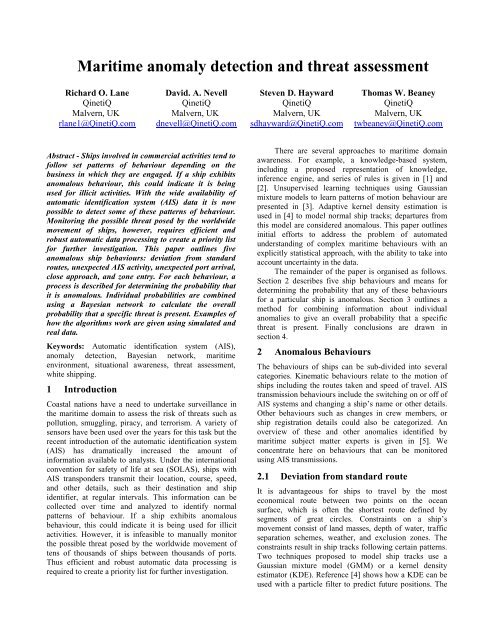
Maritime anomaly detection and threat assessment - ISIF

Maritime anomaly detection and threat assessment
Richard O. Lane
QinetiQ
Malvern, UK
rlane1@QinetiQ.com
David. A. Nevell
QinetiQ
Malvern, UK
dnevell@QinetiQ.com
Steven D. Hayward
QinetiQ
Malvern, UK
sdhayward@QinetiQ.com
Thomas W. Beaney
QinetiQ
Malvern, UK
twbeaney@QinetiQ.com
Abstract - Ships involved in commercial activities tend to
follow set patterns of behaviour depending on the
business in which they are engaged. If a ship exhibits
anomalous behaviour, this could indicate it is being
used for illicit activities. With the wide availability of
automatic identification system (AIS) data it is now
possible to detect some of these patterns of behaviour.
Monitoring the possible threat posed by the worldwide
movement of ships, however, requires efficient and
robust automatic data processing to create a priority list
for further investigation. This paper outlines five
anomalous ship behaviours: deviation from standard
routes, unexpected AIS activity, unexpected port arrival,
close approach, and zone entry. For each behaviour, a
process is described for determining the probability that
it is anomalous. Individual probabilities are combined
using a Bayesian network to calculate the overall
probability that a specific threat is present. Examples of
how the algorithms work are given using simulated and
real data.
Keywords: Automatic identification system (AIS),
anomaly detection, Bayesian network, maritime
environment, situational awareness, threat assessment,
white shipping.
1 Introduction
Coastal nations have a need to undertake surveillance in
the maritime domain to assess the risk of threats such as
pollution, smuggling, piracy, and terrorism. A variety of
sensors have been used over the years for this task but the
recent introduction of the automatic identification system
(AIS) has dramatically increased the amount of
information available to analysts. Under the international
convention for safety of life at sea (SOLAS), ships with
AIS transponders transmit their location, course, speed,
and other details, such as their destination and ship
identifier, at regular intervals. This information can be
collected over time and analyzed to identify normal
patterns of behaviour. If a ship exhibits anomalous
behaviour, this could indicate it is being used for illicit
activities. However, it is infeasible to manually monitor
the possible threat posed by the worldwide movement of
tens of thousands of ships between thousands of ports.
Thus efficient and robust automatic data processing is
required to create a priority list for further investigation.
There are several approaches to maritime domain
awareness. For example, a knowledge-based system,
including a proposed representation of knowledge,
inference engine, and series of rules is given in [1] and
[2]. Unsupervised learning techniques using Gaussian
mixture models to learn patterns of motion behaviour are
presented in [3]. Adaptive kernel density estimation is
used in [4] to model normal ship tracks; departures from
this model are considered anomalous. This paper outlines
initial efforts to address the problem of automated
understanding of complex maritime behaviours with an
explicitly statistical approach, with the ability to take into
account uncertainty in the data.
The remainder of the paper is organised as follows.
Section 2 describes five ship behaviours and means for
determining the probability that any of these behaviours
for a particular ship is anomalous. Section 3 outlines a
method for combining information about individual
anomalies to give an overall probability that a specific
threat is present. Finally conclusions are drawn in
section 4.
2 Anomalous Behaviours
The behaviours of ships can be sub-divided into several
categories. Kinematic behaviours relate to the motion of
ships including the routes taken and speed of travel. AIS
transmission behaviours include the switching on or off of
AIS systems and changing a ship’s name or other details.
Other behaviours such as changes in crew members, or
ship registration details could also be categorized. An
overview of these and other anomalies identified by
maritime subject matter experts is given in [5]. We
concentrate here on behaviours that can be monitored
using AIS transmissions.
2.1 Deviation from standard route
It is advantageous for ships to travel by the most
economical route between two points on the ocean
surface, which is often the shortest route defined by
segments of great circles. Constraints on a ship’s
movement consist of land masses, depth of water, traffic
separation schemes, weather, and exclusion zones. The
constraints result in ship tracks following certain patterns.
Two techniques proposed to model ship tracks use a
Gaussian mixture model (GMM) or a kernel density
estimator (KDE). Reference [4] shows how a KDE can be
used with a particle filter to predict future positions. The

application of a GMM to synthetic data is explained in
[3], and a comparison between GMM and KDE methods
is given in [6]. Major sea lanes, where the traffic is
highest, can be characterized using a track data-driven
approach [7]. Dividing the ocean into a number of grid
cells, with a density sufficient for a specified accuracy,
has the disadvantage that several million cells and
connections between cells would be required to model
global shipping movements [8].
An alternative model for the movement of ships at
sea uses a network of discrete nodes placed at route
decision points relating to constraints, and branches to
connect the nodes. The network model is sparse, being
branch rich and node light. This has computational
advantages as the speed of optimal route algorithms are
dominated by the number of nodes rather than the number
of branches. Since the ultimate aim is to produce a global
network, calculation time is an important issue for both
network preparation and analysis. A node-sparse network
might only need 20,000 nodes and have journeys that
involve one to ten branches rather than hundreds. This
model was first presented in [9] and is expanded here.
In the network design, each landmass in the world is
represented by a closed polygon using coastline data from
[10]. There are three types of node located on the coast:
ports, convex hull coastal points, and other coastal points
required to define journeys to ports. Offshore nodes are
added for destinations such as oil rigs, for defining the
edge of restricted routes such as traffic separation
schemes, and for observed set routes not constrained by
land. Great circle branches are generated between pairs of
nodes that are not impeded by any intervening landmass.
In addition, branches expected to be of no practical use in
route planning are excluded.
Each port is represented by a position capturing
where ships have to pass nearby on entry or exit. This is
of particular significance for ports that are either extensive
or situated some way inland on a major waterway. For
some ports, the node identifying their position was
situated on the coast, at the entrance to the dock complex
(e.g. Rotterdam), or the mouth of the river for inland
ports. In such a situation, the same destination node
represents a number of different ports.
Once the nodes and branches have been established,
Dijkstra’s algorithm is used to pre-calculate optimal
routes and costs between ports in the network. The
baseline cost function for each branch is its length but
could be augmented by canal tolls or other branch specific
features. Pre-calculation of optimal routes allows
subsequent analysis of ships’ routes to be sped up
considerably.
A ship’s journey begins and ends at a port and is
assumed to follow a route that passes through or close to a
sequence of intermediate network nodes. A complete
journey J can be described by its constituent branches
between those nodes such that J = {b 1 ,…,b n } where the b i
represent branches. In practice, it is necessary to analyze
incomplete journeys to assess whether the ship’s
behaviour has been anomalous or not. An incomplete
journey is made up of two parts: the macro part and the
micro part. The macro part consists of all branches
traversed before the previous network node. The micro
part consists of the route since the previous network node.
It is useful to divide the route in this way as the macro
route can be described with reference to the pre-defined
network, whereas the micro route, having no local nodes
with which to identify, has to use a more precise frame of
reference.
The underlying requirement is to calculate, for every
possible destination D i , the probability that the true
destination is D i , conditional on having observed the route
so far. In the particular case above this can be expressed
as
P(D i |R M ,R m ) where R M represents the macro route and R m
represents the micro route. Using Bayes’ theorem and
making the prior assumption that all ports are equally
likely destinations, it can be shown that P(D i |R M ,R m ) ∝
P(R M |D i )P(R m |D i ). P(R M |D i ) is calculated from the cost of
the route taken compared to the optimal cost. P(R m |D i ) is
calculated by comparing the ship’s heading at each
measurement point with the heading of candidate
branches. Details of these calculations are given in [9].
After every new observation of a ship’s position,
conditional destination probabilities are updated for every
destination in the network. These probabilities can be used
to assess the following two hypotheses: H 0 , the ship is
travelling to its stated destination; and H 1 , the ship is
travelling somewhere else. Implicit in the null hypothesis
H 0 is the assumption that if a ship is travelling to its stated
destination, then it will do so by a route that does not
incur unreasonable cost.
The anomaly statistic of interest is P(H 0 |r t ) where r t
is the complete route covered by the ship up to time t.
Using Bayes’ rule this can be written as
P
( )
( rt
| H0
) P( H0
)
At
: = P H0
| rt
=
.
P( rt
| H0
) P( H0
) + P( rt
| H1) P( H1)
Prior values for P(H 0 ) and P(H 1 ) are required. If it is
observed, for example, that over a representative sample
of ships’ journeys, a proportion q of them result in a ship
travelling to the stated destination D s , then P(H 0 ) could be
set to q. In this initial work, the value has been set to
0.999. This implies that P(H 1 ) should be set at 1-q. Since
H 1 includes every destination that is not the stated one this
covers n-1 destinations, where n is the total number of
possible destinations. Hence the probability that the ship
is travelling to a specific non-stated destination is (1-q)/(n-
1). For the case where there is no knowledge of the
expected destination, the use of this anomaly statistic can
be extended to a series of null hypotheses for each
possible destination D i to determine at each observation,
which of the destinations appear feasible and which
appear anomalous. At the start of a journey all
destinations will appear feasible (i.e. the A t,i value for each
hypothesized destination D i will be close to 1) but they
will be gradually whittled down as the journey progresses
and the route becomes clearer. If at any point of the

journey, every possible destination has appeared
anomalous at some previous point of the journey
(including the current point) then there remains no
feasible place for the ship to travel to and it should be
flagged up as anomalous. In other words, A t,i has fallen
below a defined threshold for every destination D i at some
time t (t is not constrained to be the same for each
destination).
A number of issues relating to real data are required
to be addressed, since certain aspects of ship behaviour
are not completely captured by the model. The method of
mapping observations onto port nodes needs to identify
which port has been reached and the precise observations
corresponding to port entry and departure. This is
important because within a port complex ships perform
maneuvers that are not modeled by the network of nodes
and branches. A circle of radius 5 km centred on each port
location was used to define each port zone. Once a ship
enters/exits a port zone, it is considered to have
reached/left that port if its speed falls below/exceeds a
tuneable threshold, set at 0.1 knot by default. For nodes
that represent inland ports the journey is considered to
have ended/started once the zone of that point is
entered/exited, regardless of the speed.
One reason for defining a node as an intermediate
step on a longer journey is that ships ought to change
direction at these points. However, real data reveals that
when ships proceed around a headland they often give it a
wide berth. When the change of heading between the
branches is slight it is only possible to be sure that the
ship’s route included that node some time after it has been
passed. It can be ensured that each node added to the
journey is correct by monitoring, at each observation,
which nodes have been passed since departure from the
previous node. These passed nodes are then analysed
further to see if any of them can be considered to have
constrained the journey. If they have, they are added to the
macro route and the micro route is reset to a new branch.
Over the course of traversing a branch, the number of
passed nodes will potentially accumulate. Some of these
are not near to the route and are not of interest since they
do not have the potential to delimit the journey. Out of the
set of passed nodes, there will be at most only two that
could possibly be added to the macro route: those that
most closely delimit the route on the port and starboard
sides. This is illustrated in Figure 1. A final check is then
made to see whether the latest measurement point has a
line of sight to the last node on the macro route (i.e. the
great circle segment connecting the point and node does
not intersect an intervening land mass). If so, a new node
is added to the macro route, else the measurement point is
added to the micro route. For the case of offshore nodes, if
a ship travels within a specified distance of the node, and
the node has been passed, then it is added to the route.
N i
B
A
Figure 1: Delimiting coastal nodes. A is the port node, B is
the starboard node, and C has not yet been reached
The deviation from standard route algorithm has been
applied to measured data of several hundred ships. An
example track of one of the ships that was considered
anomalous is shown in Figure 2. The standard route for
this ship would be to head straight across the North Sea
and dock at Bergen in Norway, but before docking the
ship instead visits two fjords. In this particular case the
ship was a cruise ship so the behaviour is not suspicious.
However, the example illustrates the ability of the
algorithm to detect ships that do not follow defined routes.
Figure 2: Ship track that deviates from a standard route
2.2 Unexpected AIS activity
Under the SOLAS regulations, ships are required to
transmit their location at regular intervals using AIS. If a
ship moves out of range of receivers, the transmitted
signals will not be detected. However, if there is a long
period of AIS silence in a good coverage area this could
be indicative of a ship having switched off its AIS
transmitter to covertly carry out illegal activities.
Conversely, if an AIS signal states a ship is in a region
where signals are not normally able to be received; this
could imply a false position has been given deliberately.
A system model for transmitters, the propagation
channel and receivers is given in [11]. Here, we give an
alternative approach to detecting the above behaviours by
building up a coverage map of the receivers. This can be
C

epresented as the probability of receiving a signal sent
from any specified location. For convenience, the area of
interest is divided into grid squares. The probability of
receiving a signal from a grid square can be calculated
using a simple ratio of detections and non-detections from
historical data. The existence of non-detection events can
be estimated by tracking ships and either projecting from
or interpolating between their positions from areas of
good coverage where detections are made.
A problem with the above method is that many grid
squares either have no or very few detection/non-detection
events, resulting in imprecise estimates of the probability.
This problem can be alleviated through the use of Bayes’
theorem. If coastal AIS receivers are being used then it is
known that the reception of AIS signals near land is more
likely than far out to sea. It is assumed, as a first
approximation, that all coastal areas are well serviced by
AIS receivers. The distance between the centre of a grid
square and the nearest coast point is calculated for every
grid square. The set of distances is grouped into bins and
the probability of receiving a signal for each of these
distance bins is calculated. This is reasonably accurate for
most distances since the number of bins is much less than
the number of grid squares. In general, the probability of
reception is a decreasing function of distance. Thus a
suitably chosen curve can be fitted to the empirical data to
obtain the probability of reception at an arbitrary distance.
The prior probability of detecting a signal in a particular
grid square is modelled using a beta distribution:
αd
−1
βd
−1
p0
( 1−
p0
)
p( p0
) = .
B( α d , β d )
The distribution parameters were set to give the
appropriate probability for the distance of the grid square
in question from the coast. The likelihood of k detections
given n detection/non-detection events is:
k n−k
p( k | p0 ) = n Ck
p0
( 1−
p0
) .
Bayes’ theorem gives the posterior probability for a
particular grid square as:
k + αd
−1
n−k+
βd
−1
p0
( 1−
p0
)
p( p0
| k)
=
.
B( k + α d , n − k + β d )
Ten days of AIS data were used to estimate the coverage
map for northern Europe. The calculated map shows the
value of using a prior distribution. In areas of high traffic
density the probability depends largely on the data
specific to each grid square. In areas of low traffic density,
the probability depends mostly on the prior.
The probability that a single unexpected AIS
reception is anomalous is simply one minus the detection
probability in the relevant grid square. The probability of
multiple unexpected AIS receptions is one minus the
product of these probabilities. To determine the
probability that a period of AIS silence is anomalous, the
ship’s last known heading and speed are used to project its
future position at sampled time intervals equal to the
interval between expected AIS recordings. The
probabilities of receiving a signal from projected grid
square locations can then be combined to give an overall
probability of not having received a signal, as a function
of time.
The above approach described the estimation of a
static coverage map averaged over a certain period of
time. However, there are predictable shifts in the ability of
AIS devices to receive signals. For example, it is easier to
detect signals in the middle of the day when the
temperature is warmer. This could be taken into account
by estimating the coverage map using one-hour segments
of data and averaging over several days. This method
could be extended to take into account seasonal variations
throughout the year. In addition to predictable patterns of
AIS detection there may be unpredictable ones. This could
be a result of unusually long detection ranges due to
ducting or short ranges in bad weather. These variations
could be mitigated through the use of constant false alarm
rate processing. Naturally the entire process could also be
applied to other types of sensor, such as satellite-based
systems, which would have a different coverage area.
2.3 Unexpected port arrival
There are two parts to this type of anomaly. The first of
these is based on types of ship and port facilities. There
are 10 main vessel types defined in Lloyd’s Register of
Ships and 11 facilities in Lloyd’s List Ports of the World.
If a ship of a particular type arrives at a port that has no
facilities to handle the ship then this could be considered
as anomalous. The implementation of a detector based on
this information is straightforward once the mapping
between facilities and vessel types is made.
The second part looks at patterns of port visitation
by ships. Over time, ships tend to visit certain ports and
not others, and the ports tend to be visited in a particular
order. Port arrivals are sequences of events that can be
characterized using a Markov model, which could be
applied to individual ships or ships in general. An
overview of Markov models for anomaly detection is
given in [12]. Briefly, a Markov model represents a
discrete-time stochastic process where the distribution
over states (ports in this case) at a particular time step
depends only on the state at the immediately preceding
step. Such a system is characterized by a transition
probability matrix and an initial probability distribution.
Each row of the transition matrix represents the
probability that a ship will move from that port to any of
the other ports. The possibility of unobserved port arrivals
is not modelled explicitly but this is instead captured by
altered probabilities in the transition matrix.
Markov model transition matrices are often
estimated by examining the proportion of times each
transition has been made in a set of training data.
However, since there is a large number of ports, and given
a limited amount of training data, the accuracy of a
transition matrix estimated this way is limited. The
situation can be improved using a Bayesian approach to
the problem. For each row of the matrix a prior
distribution is defined and the observed data are used to

update the distribution using Bayes’ theorem. The arrival
at one port out of a defined set is modelled using the
multinomial distribution. If the prior is modelled using a
Dirichlet distribution then the posterior is also a Dirichlet
distribution, with different parameters. This follows since
it is the conjugate prior of the multinomial distribution
[13].
Hidden Markov models for general anomaly
detection have been proposed in [14]. However, for the
port arrival model considered here the states are observed
directly. Thus an extra level of complexity can be
avoided.
A Markov model was applied to data of 552 ships
travelling in northern Europe over a three week period.
Out of these ships, 231 visited at least one port and 112
visited at least two ports. Many ships visited significantly
more than two ports. Port arrivals were detected using the
same methodology as that used in the deviation from
standard route anomaly detector. However, in this case the
actual locations of 610 ports were used rather than costal
nodes, so that individual inland ports could be identified.
For each ship, the geometric mean of the probability of
arriving at each of the ports in a journey was calculated.
These have been ranked and the results are shown in
Figure 3. A detector for this anomaly would set a
threshold on the mean probability; all ships with a
probability less than this threshold would be declared
anomalous.
Figure 3: Ranked mean probability of port arrivals
2.4 Close approach
A close approach event is defined as two ships being
unusually close together at sea and travelling below a
certain speed. Ships that exhibit this behaviour could
potentially be involved in the illegal transfer of goods or
people. For each measurement received from a ship, its
location, speed and heading are used to project a straightline
trajectory into the past and future over a defined time
period. Trajectories for all ships being tracked are
produced and these are used to estimate the distance
between any two ships as a function of time. The distance,
estimated location of the two ships, and the time are
recorded for the closest point of approach.
In regions near ports many ships do come into close
proximity to each other while either moored or
manoeuvring around the dock. To avoid these ships being
designated as being anomalous, a zone around each port is
used to eliminate ships from the calculation. Other
exemption zones could be defined for areas of high ship
density, such as anchorages, to avoid a high alarm rate.
One problem with implementing the distance check
directly as described above is that the number of ship
combinations is potentially huge. For example if tracking
10,000 ships (a typical number for northern Europe),
approximately 50 million ship pairs would have to be
examined. A more efficient approach is to use some form
of spatial indexing. This has been implemented by
assigning ships to grid squares and only checking pairs of
ship in the same or adjacent grid squares. This
dramatically reduces the number of checks that have to be
made. The same process of grid assignment can be applied
to exemption zones to further reduce the number of
calculations required.
Once the distance, time, and speed at closest
approach have been calculated, these are converted to a
probability for integration with the fusion process. This is
the probability of two ships having been close enough for
suspicious activities to have occurred.
2.5 Zone Entry
One event of interest is whether or not a ship has entered a
defined zone. Zones could be defined to protect
environmental areas, military installations, national
infrastructure, or to spot ships entering areas of bad
weather. In addition to actual zone entry it is also of
interest to determine the probability that a ship will enter a
zone in a given time period in the future. This would give
operations managers more time to react to a situation.
If a zone is defined as a polygon, standard
algorithms can be used to determine whether or not a
point is inside that polygon. A computational speed-up
can be gained for polygons with a large number of
vertices by first checking whether the point is in a lat/long
bounding box, then the convex hull, then the actual
polygon.
The probability that a ship will enter a zone within a
defined period of time can be calculated by assuming
some distribution for tracks projected from the current
position and determining the proportion that intersect the
zone. For this work a Gaussian distribution for heading
and speed was used, centred on the last known values and
with independent variances estimated from the variation
in historical tracks. This assumption allowed fast
processing of data. Naturally other distributions that take
into account more complicated manoeuvres, such as
slowing while turning, or navigating around land, could be
implemented using particle filters.
A parameter of interest is the estimated time of zone
entry. When a ship has actually been detected inside a
zone this can be gained by interpolating track points to
find when the zone boundary was crossed. For predicted

entry the time is calculated by averaging over the
distribution.
3 Anomaly Fusion
3.1 Threats and Behaviours
An overall threat is often manifested by a series of
individual behaviours. An example threat scenario is the
illegal exchange of goods at sea. The behaviours exhibited
by a ship undertaking this activity could include deviation
from standard route, turning off an AIS transmitter,
entering a zone known for illegal exchanges, and close
approach with another ship. Thus, the above anomaly
detectors could be used to assess the level of threat.
The degree to which behaviours are demonstrated in
real data varies between threat scenarios and, for a
particular scenario, between specific threats. There is a
need to assess what threats may be implied by the
measured data. This introduces the requirement to fuse the
evidence gathered about anomalous behaviours in order to
assess the probability of a threat being present.
3.2 Bayesian network solution
This paper proposes use of a Bayesian network to carry
out the anomaly fusion for threat assessment. The model
for threats and behaviours is similar to the threats and
signatures model of [15]. A survey of Bayesian networks
for situation assessment is given in [8].
For a given ship the output from each of the
individual anomaly detectors can be interpreted as a
likelihood: the probability that the particular behaviour of
interest actually took place, given the observations. Given
estimates of the likelihoods associated with individual
behaviours, it is possible to estimate the likelihood
associated with the threat scenario from which those
behaviours were decomposed. The process of anomaly
fusion is therefore one of combining the outputs of the
individual detectors to give a single number between zero
and one.
Let the variable representing the threat be denoted
T . If there is just one threat type under consideration T
is a binary variable and we are required to make a binary
decision between T and ¬ T . If there is more than one
threat type then we are required to make a decision
between members of the set { T 0
, T 1
, T n
}, where T 0
represents the null hypothesis that no threat is present. Let
the behaviour variables be denoted by the set
{ B , B , 1 2
B m
}. Each of these variables takes a binary
value, indicating that the behaviour is present or not. Let
the corresponding observation or detection variables be
D , D , 2
1
D m
.
denoted by the set { }
T
B 1 B 2 B 3
D 1 D 2 D 3
Figure 4: Bayesian network describing the relationship
between the detector outputs { D , D , 1 2
D m
}, and the
threat variable T
Figure 4 shows a simple Bayesian network representing
the relationship between the threat variable, T , and the
observed detector outputs { D , D , 1 2
D m
}, via the
behaviour variables { B , B , 1 2
B m
}. This network defines
a generative model for the observed detector outputs. The
model is implemented in the following stages:
1. The threat variable, T , is drawn from a categorical
distribution, with probability p ( T k
) associated with
th
the k category;
2. Given T , each of the behaviour variables is drawn
independently from a binary distribution with
p B T ), p(
B T ), , p(
B ) ;
(
1 2
m
T
probability { }
3. Given B
i
, the detector output corresponding to the
th
i behaviour,
D i
, is drawn from one of two
p D i
B and p D i
¬ B ) ,
(
i
continuous distributions, )
(
i
representing the probability of detection and the
probability of false alarm, respectively.
Using this model we require the likelihood of a threat,
T , given the observations { D , D , 1 2
D m
}, i.e.
j
p
⎡
⎢
∏
i j j
⎣ i=
1
( T
=
⎦
j
D1
, D2
Dm
) n
, (1)
m
⎡
∑ ⎢∏
⎣
m
k= 0 i=
1
⎤
p(
D T ) ⎥ p(
T )
⎤
p(
Di
Tk
) ⎥ p(
Tk
)
⎦
where
p D T ) = p(
D B ) p(
B T ) + p(
D ¬ B ) p(
¬ B T )
(
i k
i i i k
i i
i k
and the denominator is chosen to ensure that
n
∑
k = 0
p(
Tk D1 , D2,
D m
) = 1. Let p D i
B ) , the probability
(
i
of detection, be represented by some assumed density

(
i
(
i
function f D ) and let p D i
¬ B ) , the probability of
false alarm be represented by density function g ( Di
) .
Defining w = p(
B T ) , w
~
= p(
¬ B T ) , we get
j
1
2
i, k
i k
p( T D , D D )
m
=
n
i, k
i k
m
∏ ( wi,
j
f ( Di
) + w~
i,
j
g(
Di
))
⎡
⎢
⎣
⎡
i=
1
m
∑ ⎢∏ ( w
k
f Di
+ w
k
g Di
)
i ,
( ) ~
i ,
( )
⎣
k = 0 i=
1
⎤
⎥ p(
T
j
)
⎦ .
⎤
⎥ p(
Tk
)
⎦
In order to evaluate (2), prior probabilities for the
occurrence of each category of threat
{ p( T0 ), p(
T1
), , p(
Tn
)}
must be specified. Clearly
p ( T 0
) must satisfy
n
0
) = 1−∑
p(
T k
)
k=
1
p( T
.
It is necessary to specify the density functions f ( Di
) and
g ( Di
) . In the absence of suitable data with ground-truth
that would allow f ( Di
) and g ( Di
) to be estimated for
each detector, a reasonable approach is to assume that
f ( Di ) = f D , ∀ , g( Di ) = g( D) , ∀i
. Finally the
( ) i
conditional probabilities defined by the weights { }
must also be specified.
3.3 Using detector outputs
w i,
k
For cases where the densities of the detector outputs
conditional on the behaviours f ( Di
) and g ( Di
) are
unknown, but estimates of the posterior probabilities of
behaviours are available, then we can write:
P(
T | D ,…
D ) ≈
1
In this equation
m
∑
P(
T | B ,…
B )
∏
1 m
B1
,…
B m
i=
1
∑
m
∏
∏
k
k= 0 i=
1
m
P(
B | D )
i
i
k
i
(2)
(3)
P(
T ) P(
Bi
| T )
i=
1
P( T | B1
,… Bm
) = n
m
(4)
P(
T ) P(
B | T )
and we have assumed independence of the behaviours and
detector outputs:
m
1
, Bm
| D1
, Dm
) = ∏ P(
Bi
| Di
)
i=
1
P( B …
… .
Equations (3) and (4) are of use if we interpret the outputs
of the anomaly detectors as pseudo probabilities (i.e.
confidences) of behaviours being present, since these can
then be used as approximations to the P B i
| D ) . If the
(
i
actual likelihoods P ( D i
| Bi
) are known it’s better to
use them in (1).
3.4 Numerical example
We give here a simple numerical example to illustrate the
principle of the Bayesian network approach to threat
assessment. In this example there is one threat and two
behaviours. We compare the properties of the detection
statistic from (2) with the estimates of
P ( T | D1 ,… Dm
) from (3), for varying values of D
1
and
D
2
. Parameters for the problem are given in Table 1 and
results are shown in Figure 5 and Figure 6. As expected,
the overall probability of threat is high when either of the
behaviour detector outputs is high. However, it is
interesting to note the difference in output of the two
approaches. The determined probability of threat in Figure
6 is generally higher using (3) than when using (2). Thus
care should be taken when interpreting outputs of anomaly
detectors as probabilities.
D2
P (T ) 0.01
p ( T ) 1
0.95
p ( T ) 2
0.95
f (D) 2D , 0 ≤ D ≤ 1
g (D) 2 − 2D
, 0 ≤ D ≤ 1
Table 1: Parameters used in data fusion examples
0
0.1
0.2
0.3
0.4
0.5
0.6
0.7
0.8
0.9
1
0 0.2 0.4 0.6 0.8 1
D1
Figure 5: Probability that a threat is present as a function
of the detector outputs using (2)
0.7
0.6
0.5
0.4
0.3
0.2
0.1
P(T|D1,D2)

D2
0
0.1
0.2
0.3
0.4
0.5
0.6
0.7
0.8
0.9
1
0 0.2 0.4 0.6 0.8 1
D1
Figure 6: Probability that the threat is present as a function
of the detector outputs using (3)
4 Conclusion
This paper has presented initial work on algorithms for
calculating the probability that any of five specific
anomalies is present in ship AIS data. These algorithms
have been applied to real data and a selection of results
has been shown. A general Bayesian network-based
method for taking these individual anomalies and
determining the probability of a higher-level threat has
been outlined. Simulated data has been used to illustrate
the approach. Future work should involve a discussion
with subject matter experts to help determine the
numerical connection between specific behaviours and
threats. The Bayesian network model could then be
applied to real data.
References
[1] J. Roy, Automated Reasoning for Maritime Anomaly
Detection, NATO Workshop on Data Fusion and
Anomaly Detection for Maritime Situational Awareness,
La Spezia, Italy, 15-17 September 2009.
[2] J. Roy and M. Davenport, Categorization of
Maritime Anomalies for Notification and Alerting
Purpose, NATO Workshop on Data Fusion and Anomaly
Detection for Maritime Situational Awareness, La Spezia,
Italy, 15-17 September 2009.
[3] D. Garagic, B. J. Rhodes, N. A. Bomberger, and M.
Zandipour, Adaptive Mixture-Based Neural Network
Approach for Higher-Level Fusion and Automated
Behavior Monitoring, NATO Workshop on Data Fusion
and Anomaly Detection for Maritime Situational
Awareness, La Spezia, Italy, 15-17 September 2009.
[4] B. Ristic, B. La Scala, M. Morelande, N. Gordon,
Statistical analysis of motion patterns in AIS Data:
Anomaly detection and motion prediction, 11th
International Conference on Information Fusion, Cologne,
Germany, July 2008.
0.7
0.6
0.5
0.4
0.3
0.2
0.1
P(T|D1,D2)
[5] J. van Laere and M. Nilsson, Evaluation of a
workshop to capture knowledge from subject matter
experts in maritime surveillance, 12th International
Conference on Information Fusion, Seattle, WA, USA, 6-
9 July 2009.
[6] R. Laxhammar, G. Falkman, E. Sviestins, Anomaly
detection in sea traffic – a comparison of the Gaussian
mixture model and kernel density estimators, 12th
International Conference on Information Fusion, Seattle,
WA, USA, 6-9 July 2009.
[7] A. Baldacci, S. Rolla, C. Carthel, Maritime traffic
characterization with the Automatic Identification System,
NATO Workshop on Data Fusion and Anomaly Detection
for Maritime Situational Awareness, La Spezia, Italy, 15-
17 September 2009.
[8] R. Laxhammar, Artificial intelligence for situation
assessment, MSc Thesis, Royal Institute of Technology,
Stockholm, Sweden, 2007.
[9] D. Nevell, Anomaly detection in white shipping,
Mathematics in Defence 2009, Farnborough, Hampshire,
UK, 19 November 2009.
[10] National Geophysical Data Centre coastline
extractor (http://rimmer.ngdc.noaa.gov)
[11] A.Baldacci, M. Cappelletti, C.Carthel, S.Coraluppi,
AIS transponder anomaly detection for Maritime
Situational Awareness, NATO Workshop on Data Fusion
and Anomaly Detection for Maritime Situational
Awareness, La Spezia, Italy, 15-17 September 2009.
[12] N. Ye, A Markov chain model of temporal behaviour
for anomaly detection, IEEE Workshop on Information
Assurance and Security, US Military Academy, West
Point, NY, 6-7 June 2000.
[13] J.-M. Bernard, An introduction to the imprecise
Dirichlet model for multinomial data, International
Journal of Approximate Reasoning, 39:123-150, 2005.
[14] J. Barker, R. Green, P. Thomas, G. Brown, D.
Salmond, A Bayesian information fusion decision support
tool for the identification of difficult targets, Mathematics
in Defence 2009, Farnborough, Hampshire, UK, 19
November 2009.
[15] J. M. Beaver, R. A. Kerekes, J. N. Treadwell, An
information fusion framework for threat assessment, 12th
International Conference on Information Fusion, Seattle,
WA, USA, 6-9 July 2009.