Multiple Sensor Multiple Object Tracking With GMPHD Filter - ISIF

Multiple Sensor Multiple Object Tracking With
GMPHD Filter
Nam Trung Pham, Weimin Huang
Institute for Infocomm Research, Singapore
Email: {stuntp,wmhuang}@i2r.a-star.edu.sg
S. H. Ong
Department of Electrical and Computer Engineering
National University of Singapore
Email: eleongsh@nus.edu.sg
Abstract— Tracking objects using multiple sensors is more
efcient than those using one sensor. In this paper, we proposed
a method to fuse data from multiple sensors in Gaussian mixture
probability hypothesis density lter. This method can avoid the
data association problem in multi-sensor multi-object tracking.
Moreover, it is more reliable and less computational than particle
probability hypothesis density lter for multi-sensor multi-object
tracking. We demonstrated the efcient of the approach by
applications such as bearing and range tracking, and multiple
speaker tracking.
Keywords: Random nite set, Gaussian mixture probability
hypothesis density, bearing and range tracking, speaker
tracking.
I. INTRODUCTION
Multi-sensor multi-object tracking has received many attentions
in recent years. In the multi-sensor tracking system,
data fusion techniques combine data from multiple sensors
to obtain the state estimates of objects. The performance of
the tracking system can be improved by fusing data from
multi-sensor [1], [2]. However, the multi-sensor multi-object
tracking problem is challenging. These challenges are varying
number of objects, complexity in data association between
observations and objects.
Many data fusion approaches have been developed for
multi-sensor multi-object tracking in recent years. Two main
approaches are sensor-level fusion and feature-level fusion.
These approaches correspond to two levels of data association.
In the sensor-level fusion approach, observations from objects
are used to track objects at each sensor. These tracks are
associated and fused to obtain the state estimates by using
methods such as interaction multiple model [3], joint probability
data association [4], multiple hypothesis tracking [5].
Some people employed the sensor-level fusion approach for
tracking [1], [2], [3], [6]. The second approach is feature-level
fusion. In this approach, all observations from multiple sensors
are sent to the fusion center. Then, the fusion center associates
these observations with objects to obtain state estimates. Some
methods used this approach for multi-sensor multi-object
tracking [7], [8]. However, up to now, methods that are based
on two these approaches are computationally intensive because
they have to solve the data association problem.
Recently, random set approaches gave a new direction
for multi-sensor multi-object tracking. Here, the states of
objects are represented as random sets. Using this model,
the birth and death of objects can be described in the tracking
algorithm. Moreover, measurements and false alarms are
also represented as random sets in the observation model.
Mahler [9] employed the random set framework to propose a
probability hypothesis density (PHD) lter. This method can
avoid the data association between observations and objects.
Some implementations of PHD lter are proposed by using the
sequential Monte Carlo (SMC) method [10], [11]. Especially,
the implementation in [10] has the convergence proof, and
it is called particle PHD lter. In these implementations, the
state estimates are extracted from particles representing the
posterior intensity by using clustering techniques. Vo [12]
proposed a close-form for PHD lter with assumptions on
linear Gaussian system. It is called GMPHD lter. This method
reduced a lot computation compared with particle PHD lter.
For multi-sensor multi-object tracking, there are some methods
to fuse data from multi-sensor in random set approaches
such as multiplication likelihood function from sensors [13] or
sequential sensor updating [9], [14]. These methods can track
varying number of objects with multi-sensor. However, they
are implemented based on sequential Monte Carlo, so they
need a lot computation.
In this paper, we proposed a method for multi-sensor multiobject
tracking based on GMPHD lter. We extended the
GMPHD lter from one sensor to multi-sensor. The way we
choose to fuse data from multi-sensor is sequential sensor
updating in [9], [14]. Our method can collaborate information
from multiple sensors and avoid the data association
between observations and objects. In addition, we applied our
method in bearing and range tracking, and multiple speaker
tracking. For bearing and range tracking, we proved that
our method can fuse data from multiple sensors to obtain
the better performance than tracking multi-object with one
sensor. For multiple speaker tracking, our method reduced a lot
computation compared with methods using data association or
particle PHD lter in multiple speaker tracking such as [13],
[14] and [15]. Moreover, our method has reliable estimations
of speaker positions.
The paper is organized as follows. In the section II, we
formulate the multi-sensor multi-object tracking problem in
random nite set model. In the section III, the PHD lter
approach is reviewed. In section IV, we extend GMPHD lter
from one sensor to multi-sensor and implementation issues are
discussed. Finally, some experimental results in bearing and

ange tracking, and multiple speaker tracking are presented in
the section V.
II. PROBLEM FORMULATION
The multi-sensor multi-object tracking problem can be
modelled by random nite set (RFS) framework. Let X be
the single object state space then multiple object state at
time k is presented by X k = fx k;1 ; x k;2 :::; x k;Nk g 2 F(X ),
where F(X ) denotes the collection of all nite subsets of the
space X . For a multi-object state X k 1 at time k 1, each
x k 1 2 X k 1 can continue to exist at time k with probability
p S;k or die at time k with probability (1 p S;k ). Let S k (x k 1 )
denote the object that is the transition from x k 1 at time k on
condition that the object is survived and let B kjk 1 (x k 1 ) be
objects spawned at time k from an object with previous state
x k 1 . Let k be RFS of spontaneous births at time k and
can be determined by using the assumption of spontaneous
birth models. Given a multi-object state X k 1 at time k 1,
the multi-object state X k at time k is given by union of the
surviving objects and new objects,
X k =
h[ h[ i
Sk (x k 1 )i
[ Bkjk 1 (x k 1 )
[ [ k] (1)
The RFS X k encapsulates all aspects of multi-object tracking
problem, such as time varying number of objects, object
motion.
Similarly, let Z i be the measurement space of single object
at sensor i then measurements collected at sensor i time k is
Zk i 2 F(Zi ). A given object state x k 2 X k is either detected
with probability p D or missed with probability (1 p D ).
Conditional on detection, the measurement from x k at sensor
i is dened by the RFS i k (x k). The sensor i also can receive
a set of clutters Ck i . So, given a multi-object state X k at time
k, the measurement set from sensor i at time k is formed by
the union of object generated measurements and clutters,
" #
[
Zk i = i k(x k ) [ Ck i (2)
x k 2X k
Assuming that we have Q sensors, the RFS of measurements
at time k is modelled by
h
i
Z k = Zk; 1 Zk; 2 : : : ; Z Q k
(3)
The RFS Z k encapsulates all sensor characteristics such as
measurement noise, sensor eld of view, clutter.
The multi-sensor multi-object tracking can be posed as
follows: given set of measurement Z 1:k collected from sensors
up to time k, the problem is to nd ^X k is expectation or
maximization of the posterior density function p(X k jZ 1:k ).
III. PROBABILITY HYPOTHESIS DENSITY APPROACH
In multiple object tracking problem, we usually need to
obtain the posterior density p(X k jZ 1:k ). When the number
of object increases, the multiple object state space become
large. Hence, it is difcult to obtain the posterior density function.
Fortunately, this density function can be approximately
recovered from the probability hypothesis density (PHD) [9].
The PHD is dened as follows. For a random nite set X on
X with probability distribution P , the PHD is the density v(x)
such that for each region S X , the integral of v over region
S gives the expected number of elements of X that are in S,
Z
Z
j X \ S j P (dX) = v(x)dx; (4)
Thus, instead of estimating states of objects from posterior
density, we can estimate them by investigating peaks of PHD.
It helps to reduce from searching in multiple object state space
to single object state space.
IV. GAUSSIAN MIXTURE PROBABILITY HYPOTHESIS
DENSITY FILTER IN MULTI-SENSOR MULTI-OBJECT
A. Assumptions
TRACKING
First, there are some assumptions. The transition function
of each object follows a linear Gaussian model, i.e.,
f kjk 1 (xj) = N(x; F k 1 ; Q k 1 ) (5)
where N(:; m; P ) denotes a Gaussian density with mean m
and covariance P , F k 1 is the state transition matrix, Q k 1
is the process noise covariance. There are Q sensors, the
likelihood function at each sensor is also a linear Gaussian
model, i.e.,
g i k(zjx) = N(z; H i kx; R i k) (6)
where H i k is the observation matrix of the sensor i, and Ri k is
the observation noise covariance of the sensor i. The survival
and detection probabilities are
S
p S;k (x) = p S;k (7)
p D;k (x) = p D;k (8)
The intensity of the spontaneous birth RFS is
J ;k
X
k (x) =
i=1
w (i)
;kN(x; m(i)
;k ; P (i)
;k ) (9)
where J ;k is the number of birth Gaussian components at
time k, and w (i)
;k
is the weight for i-th Gaussian component.
The posterior intensity at time k 1 is a Gaussian mixture of
the form
v k 1 (x) =
J
X k 1
i=1
w (i)
k 1
N(x; m(i)
k 1 ; P (i)
k 1 ) (10)
where J k 1 is the number of Gaussian components of posterior
intensity at time k 1, and w (i)
k 1
is the weight for i-th
Gaussian component.
B. GMPHD lter with one sensor
Vo [12] proposed a closed form expression of the PHD
lter for linear Gaussian multi-object tracking, called the
Gaussian mixture probability hypothesis density lter. Under
assumptions in IV-A, the initial prior intensity is a Gaussian
mixture, the posterior intensity at any subsequent time step is

1 (x) with measurement set Z1 k by equation (13) to obtain
also a Gaussian mixture. In the case there is one sensor, this the PHD at time k sensor 1, vk 1(x). Because v k 1(x) is a
method can be employed.
Gaussian mixture, vk 1 (x) is also a Gaussian mixture and has
In what follows, we outline the GMPHD lter with assumptions
the form
vkjk 1 Jk 1 = (J k 1 + J ;k )(1 + jZkj) 1 (20)
there are no spawning objects. (In the case there
JkX
1
are spawning objects, the prediction equation is modied
vk(x) 1 = w (i)
1;kN(x; m(i)
1;k ; P (i)
1;k ) (14)
by adding Gaussian components representing for spawning
i=1
objects. The details is in [12]).
Now, at the sensor 2, we use vk 1 (x) as the predicted PHD for
Under assumptions in IV-A, the predicted intensity to time the sensor 2 and in the similar way to (13), we have
k is given by
v
v kjk 1 (x) = v S;kjk 1 (x) + k (x) (11)
k(x) 2 = (1 p D;k )vk(x) 1 + X
v D;k (x; z) (15)
z2Zk
2
where
So, v
J
X k 1
k 2 (x) also have the Gaussian mixture form.
v S;kjk 1 (x) = p S;k w (j)
k 1N(x; m(j)
S;kjk 1 ; P (j)
S;kjk 1 );
JkX
2
j=1
vk(x) 2 = w (i)
2;kN(x; m(i)
2;k ; P (i)
2;k ) (16)
m (j)
S;kjk 1
= F k 1 m (j)
k 1 ;
i=1
P (j)
S;kjk 1
= Q k 1 + F k 1 P (j)
k 1 F k T We repeat this process with Q sensors. At the Qth sensor, we
1:
obtained v Q k
(x), and it has the form
Because v S;kjk 1 (x) and k (x) are Gaussian mixtures,
J
v kjk 1 (x) can be expressed as a Gaussian mixture of the form
kX
Q
v Q k (x) = w (i)
Q;kN(x; m(i)
Q;k ; P (i)
Q;k ) (17)
J kjk
X 1
v kjk 1 (x) = w (i)
kjk 1N(x; m(i)
kjk 1 ; P (i)
i=1
kjk 1 ) (12) The PHD for the multi-sensor multi-object posterior density
i=1
will be
Then, the posterior intensity at time k is also a Gaussian
v k (x) = v Q k
(x) (18)
mixture, and is given by
v k (x) = (1 p D;k )v kjk 1 (x) + X
The number of objects is estimated by
v D;k (x; z) (13)
Z
z2Z k ^N kjk = v k (x)dx
where
J kjk
X 1
Z JkX
Q
v D;k (x; z) = w (j)
k
(z)N(x; m(j)
kjk ; P (j)
kjk );
= w (i)
Q;kN(x; m(i)
Q;k ; P (i)
Q;k )dx
j=1
i=1
w (j)
k (z) = p D;k w (j)
kjk 1 q(j) k
(z)
JkX
Q
P
= w (i)
Jkjk
k (z) + p
1
D;k l=1
w (l)
kjk 1 q(l) k
(z);
Q;k
i=1
(19)
q (j)
k (z) = N(z; H km (j)
kjk 1 ; R k + H k P (j)
kjk 1 HT k ); So, the properties of the Gaussian mixture in the case of
m (j)
kjk
= m (j)
kjk 1 + K(j) k (z H km (j)
kjk 1 );
multi-sensor is similar with one sensor case. This means in the
multi-sensor multi-object tracking problem, under assumptions
P (j)
kjk
= [I K (j)
k
H k]P (j)
kjk 1 ;
in IV-A, the initial prior intensity of multi-sensor multi-object
tracking is a Gaussian mixture, the posterior intensity for
K (j)
k
= P (j)
kjk 1 HT k (H k P (j)
kjk 1 HT k + R k ) 1 : asynchronous sensor fusion method at any subsequent time
C. GMPHD lter with multi-sensor
step is also a Gaussian mixture.
When there are many sensors, we propose a method to D. Implement issues
solve by using GMPHD lter sequentially at each sensor. The
The state estimations of objects are the means of Gaussian
algorithm is described as follows.
components that have high weights (above 0.5) in v
With assumptions in IV-A, at time k 1 we have
k (x). This
estimation method is more efcient than particle PHD lter.
J
X k 1
Because in particle PHD lter, we obtain the number of objects
v k 1 (x) = m (i)
k 1N(x; w(i)
k 1 ; P (i)
k 1 )
^N kjk then partition particles into ^N kjk clusters. If ^N kjk is not
i=1
First, we used assumptions on state equation (5), measurement
corrected, then the tracking performance will be affected.
Now, we investigate the number of Gaussian components in
equation (6) and v k 1 (x) to predict the intensity vkjk 1 1 (x) v k (x). At the rst sensor, the number of Gaussian components
at the sensor 1 by using the equation (11). Then we update is

At the second sensor, the number of Gaussian components is
Jk 2 = Jk(1 1 + jZkj)
2
= (J k 1 + J ;k )(1 + jZkj)(1 1 + jZkj) 2 (21)
So, the number of Gaussian components in v k (x) is
J k = J Q k
= (J k 1 + J ;k )(1 + jZkj) 1 (1 + jZ Q k
j) (22)
The number of Gaussian components in GMPHD with multisensor
increases so much with the time that leading to high
computation. So, at each time, methods to reduce the number
of Gaussian components are required. There are some rules to
reduce the number of Gaussians, such as Gaussian components
that have small weights will be cut, Gaussian components that
are close together will be merged into one Gaussian, and if the
number of Gaussian components is over a threshold L, rst
L Gaussian components with high weights will be chosen for
propagating in the next iteration [12].
V. EXPERIMENTAL RESULTS
A. Gaussian mixture probability hypothesis density lter with
multi-sensor for bearing and range tracking
First, we consider a bearing and range tracking application
to demonstrate the effectiveness of GMPHD lter with multisensor.
There are objects that appeared and disappeared at
different times. Each object has the survival probability p S;k =
0:99 and follows a nonlinear nearly constant turn model [12]
in which the target state takes the form x k = y T k ; ! k T
,
where y k = [p x;k ; p y;k ; _p x;k ; _p y;k ] T is the coordinate (x; y)
and velocity in each dimension of object, and ! k is the turn
rate. The state dynamic equations are given by
y k = F (! k 1 )y k 1 + G! k 1 ; (23)
! k = ! k 1 + u k 1 ;
where = 1s, ! k N (; 0; 2 wI 2 ), w = 15 m/s 2 , u k
N (; 0; 2
u), and u = =180 rad/s. 3
sin! 1 cos!
1 0
!
!
1 cos! sin!
F (!) = 6 0 1 !
! 7
4 0 0 cos! sin! 5 ,
0 0 sin! cos!
2 3
G =
6
4
2
2
0
0 2
2
0
0
7
5
We assume no spawning and that the spontaneous birth RFS
is Poisson with intensity
where
k (x) = 0:1N (x; m ; P )
m = [0; 0; 2000; 0; 0] T ;
P = diag([2500; 2500; 2500; 2500; (6=180) 2 ] T ):
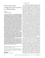
Fig. 1. Position (x; y) of targets with measurements from sensor 1
Each object has a probability of detection p D;k = 0:98.
Observations consist of bearing and range measurements from
2 sensors. The position of the sensors are
p 1 s = [0; 0] (24)
p 2 s = [1000; 1000] (25)
The observation model at sensor i is given by
2
3
px;k p
arctan
i s;x
zk i = 4
p y;k p
q
i s;y 5 + k ; (26)
(p x;k p i s;x) 2 + (p y;k p i s;y) 2
where k N(:; 0; R k ) with R k = diag([ 2 ; 2 r] T ), =
=30 rad/s and r = 10 m. The clutter RFS follows the uniform
Poisson model over the surveillance region [ =2; =2]
rad [0; 3000] m, with c = 1:1 10 3 radm 1 (i.e., an
average of 10 clutter returns on the surveillance region). The
pruning parameters for the GMPHD lters are T = 10 5 ,
merging threshold U = 4, and maximum number of Gaussian
components J max = 100. (More details on these parameters
are in [12]).
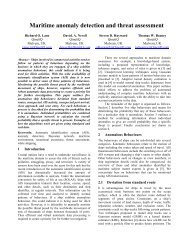
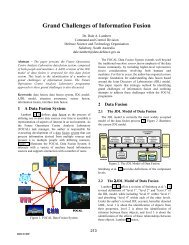
Figure 1 and 2 show the position estimations with measurements
from sensor 1 and 2 respectively. Because of the
high clutter and high noise, there are some errors in the
lter outputs. Figure 3 shows the position estimations with
GMPHD method. The performance outperformed with using
one sensor. This is because the results from sensor 1 is the
good prediction for sensor 2. Thus, the information from both
sensors is collaborated to give the state estimates.
B. Gaussian mixture probability hypothesis density lter for
multiple speaker tracking
Second, we tested the GMPHD lter in multiple speaker
tracking. We simulated an acoustic room to test the performance
of GMPHD in tracking multiple speakers. The
dimensions of the room are 3m 3m 2.5m. There are four

delay of arrival measurement (TDOA) z q k
is measured from the
q-th microphone pair at time k. The measurement equation is
z q k
= T q (x k ) + v q k
; q = 1; :::; Q (28)
T q (x k ) = kx k p 2;q k kx k p 1;q k
(29)
c
where p i;q is the position of microphone i of pair q, c is the
speed of sound, and v q k
N(0; 4 10 9 ) is uncorrelated
noise. Because the measurement equation (28) is not linear
Gaussian, we need to approximate the linear system by using
unscented transform in GMPHD lter [12]. Each speaker has a
probability of survival at time k is p S;k = 0:95, the probability
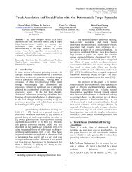
of detection is p D;k = 0:7. To extract the TDOA for multiple
speakers, we applied the method from [13]. Figure 4 shows
an example to collect TDOA measurements at a microphone
pair (for example microphone pair 2).
Fig. 2. Position (x; y) of targets with measurements from sensor 2
Fig. 4.
GCC TDOA measurements
Fig. 3.
Position (x; y) of targets with fusion method
microphone pairs, each of them has an inter-sensor spacing of
0.5m. The speaker sources are all female. The acoustic image
method [16] was used to simulate the room impulse responses.
The reverberation time of the room impulse responses is about
T 60 = 0:15s. The speech signal to noise ratio is about 20dB.
There are 60 frames. The time frame length for measuring
TDOA is 256ms, and they are non-overlapping. There are two
speakers. They appeared and disappeared at different times.
Let x k be the state of a speaker at time k. Here, the state
is the position (x; y) of speaker. We assume that the dynamic
moving equation can be given
x k = Ax k 1 + w k (27)
where A = [I] and w k N([0; 0]; diag([0:01; 0:01])). This
means the average distance from the previous time k 1 to
k of a speaker is about 10 cm. Given a speaker x k , the time
Figures 5 and 6 show the multi-speaker tracking performance
of particle PHD lter [14]. Because of the unreliable in
clustering technique, the state estimaties are affected. Figures
7 and 8 show the multi-speaker tracking performance of our
method. This performance is better than particle PHD lter. In
most of the time that two persons speak simultaneously, our
method can give reliable estimations. This is because GMPHD
lter does not depend on clustering techniques. The state
estimates are extracted from means of Gaussian components
that have high weights.
The above result is the performance for one trial. To
measure the average performance, we used the performance
measurement from [13]. It includes the probability of correct
speaker number, expected absolute error on the number of
speaker and conditional mean distance error by Wasserstein
distance. The probability of correct speaker number is dened
by
P (j ^X k j = jX k j) (30)
where ^X k is the estimation of multi-speaker state and X k is
ground-truth. The expected absolute error on the number of
speaker is
E(j ^X k j jX k j) (31)

Fig. 5.
Number of speakers by particle PHD lter
Fig. 7.
Number of speakers by our method
Fig. 6.
Position (x; y) of speakers with particle PHD lter
Fig. 8.
Position (x; y) of speakers by our method
When j ^X k j = jX k j, the Wasserstein distance between ^X k and
X k is dened as follows
d(X k ; ^X k ) = inf
C
0
@ X
x i2X k
11=P
X
d(x i ; ^x j ) P A
^x j2 ^X k
(32)
where C represents an j ^X k j jX k j. The conditional mean
distance error is dened
Efd(X k ; ^X k )jcorrect speaker number estimateg (33)
We tested the performance with 500 trials. Each trial is a
new signal and a new TDOA measurement set. Figures 9
and 10 show the probability of correct speaker number and
expected absolute error in estimation of number of speaker
compared between our method and particle PHD lter. Our
method is more accurate than particle PHD lter. The main
error in our method occur due to TDOA measurements are
not reliable when there are two people speaking at the same
time. Figures 11 shows the conditional mean distance error of
speaker tracking. It is more stable than particle PHD lter.
VI. CONCLUSIONS
Multi-sensor multi-object tracking is a challenging problem.
In this paper, we employed GMPHD lter for multi-sensor
multi-object tracking. The sequential sensor updating was used
to fuse data from multi-sensor in the GMPHD lter. We proved
that our method can work well for multi-sensor in the bearing
and range multi-object tracking. Moreover, we demonstrated
that GMPHD lter is more efcient than particle PHD lter
in multiple speaker tracking.
VII. ACKNOWLEDGEMENT
The authors would like to thank Prof. Ba Ngu Vo at
Melbourne University for his helps and fruitful discussions.
This work is partially supported by EU project ASTRALS
(FP6-IST-0028097).
REFERENCES
[1] G. Wang, R. Rabenstein, N. Strobel, and S. Spors, “Object localization
by joint audio-video signal processing,” in Vision Modelling and
Visualization, Germany, 2000.
[2] P. J. Escamilla-Ambrosio and N. Lieven, “A multiple-sensor multipletarget
tracking approach for the autotaxi system,” in IEEE Intelligent
Vehicles Symposium, Italy, 2004.

Fig. 9.
Probability of correct speaker number
Fig. 11.
Conditional mean distance error of multi-speaker tracking
tracking of sound sources using beamforming and particle ltering,” in
Proc. IEEE Int. Conf. Acoust., Speech, Signal Processing (ICASSP-06),
France, 2006.
[16] J. Allen and D. Berkley, “Image method for efciently simulating small
room acoustic,” Journal of the Acoustical Society of America, vol. 65,
pp. 943–950, 1979.
Fig. 10.
Absolute error on the number of speaker
[3] Z. Ding and L. Hong, “Development of a distributed IMM algorithm
for multi-platform multi-sensor tracking,” in International Conference
on Multisensor Fusion and Intergration for Intelligent Systems, USA,
1996.
[4] Y. Bar-Shalom and T. E. Fortmann, Tracking and data association. San
Diego: Academic Press, 1988.
[5] D. Reid, “An algorithm for tracking multiple targets,” IEEE Transaction
Automatic Control, vol. 24, no. 6, pp. 84–90, 1979.
[6] K. Chang, C. Chong, and Y. Bar-Shalom, “Joint probabilistic data association
in distributed sensor networks,” IEEE Transaction on Automatic
Control, vol. 31, no. 10, 1986.
[7] L. Y. Pao and S. D. O'Neil, “Multisensor fusion algorithms for tracking,”
in Proceeding of American Control Conference, USA, 1993.
[8] L. Cheny, M. J. Wainwright, M. Cetiny, and A. S. Willsky, “Multitargetmultisensor
data association using the tree-reweighted max-product
algorithm,” in SPIE AeroSense Conference, USA, 2003.
[9] R. Mahler, “Multi-target Bayes ltering via rst-order multi-target
moments,” IEEE Trans. on Aerospace and Electronic Systems, vol. 39,
no. 4, pp. 1152–1178, 2003.
[10] B. N. Vo, S. Singh, and A. Doucet, “Sequential Monte Carlo methods
for Bayesian multi-target ltering with random nite sets,” IEEE Trans.
Aerospace and Electronic Systems, vol. 41, no. 4, pp. 1224–1245, Oct
2005.
[11] T. Zajic and R. Mahler, “A particle system implement of the PHD multitarget
tracking lter,” in Signal Processing, Sensor Fusion and target
Recognition XII, SPIE Proc, 2003, pp. 291–299.
[12] B. N. Vo and W. K. Ma, “The Gaussian mixture probability hypothesis
density lter,” IEEE Transaction Signal Processing, vol. 54, no. 11,
2006.
[13] W. K. Ma, B. Vo, S. Singh, and A. Baddeley, “Tracking an unknown
time-varying number of speakers using TDOA measurements: a random
nite set approach,” IEEE Trans Signal Processing, vol. 54, no. 9, 2006.
[14] B. N. Vo, S. Singh, and W. K. Ma, “Tracking multiple speakers with
random sets,” in ICASSP, Montreal, Canada, 2004.
[15] J. M. Valin, F. Michaud, , and J. Rouat, “Robust 3D localization and