Towards Wiki-based Dense City Modeling - Institute for Computer ...

atio of about 10:1). Consequently, view pairs with a large
overlap and appropriate triangulation angles are preferable.
Hence, we rank the views with sufficient overlap according
to the following score:
A H
A median(ψ(α i)), (7)
where α i is the angle between corresponding rays and ψ(·)
is a unimodal weighting function with its maximum at α 0 .
We choose ψ as
ψ(α) = α 2 e −2α/α0 . (8)
The two views with highest scores are taken as sensor
views.
Dense depth estimation depends heavily on the quality
of the provided epipolar geometry. In order to reduce the
influence of inaccuracies in the estimated poses on the depth
maps, and to increase the performance, multi-view stereo
is applied on downsampled images (512 × 384 pixels for
4 : 3 format digital images). Matching cost computation
and scanline optimization for view triples (one key view and
two sensor views) take about 3s on a GeForce 7800GS.
The set of depth maps provides 2.5D geometry for each
view. These depth maps are subsequently fused into a common
3D model using a robust depth image integration approach
[25]. This method results in globally optimal 3D
models according to the employed energy functional, but it
operates in batch mode. The incorporation of this step is
the major reason for dense geometry generation to be an offline
process. The result obtained by depth map fusion for
the dataset depicted in Figure 2 (augmented with per-vertex
coloring) is shown in Figure 3.
5. Results
We tested our system on different image collections,
varying from a few hundred to thousands of pictures. All
images are calibrated with the method described in Section
2. The calibration precision (i.e. the final mean reprojection
error) ranges from 1/20 to 1/7 pixel. Our largest
test set is a database containing about 7000 street-side images
taken with four compact digital cameras from different
manufacturers. The images are captured at different days
under varying illumination conditions. Furthermore, the
images are only partially ordered. The size of the source
images varies from two to seven Megapixel. In order to remove
compression artefacts, the supplied images are resampled
to the half resolution for further processing. Adding
an image to the view network takes approximately half a
minute, most of the time is spend on exhaustive matching
and bundle adjustment. Average run-times required for each
step are listed in Table 1.
In all our tests we use a pre-trained generic vocabulary
tree of about 7 × 10 5 leaf nodes for searching the image
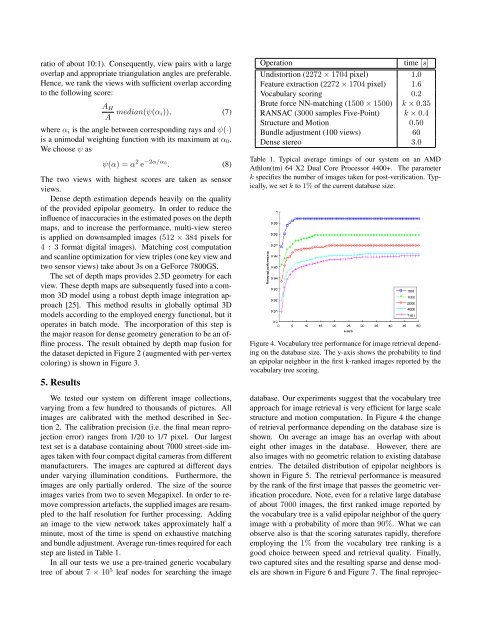
Operation
time [s]
Undistortion (2272 × 1704 pixel) 1.0
Feature extraction (2272 × 1704 pixel) 1.6
Vocabulary scoring 0.2
Brute force NN-matching (1500 × 1500) k × 0.35
RANSAC (3000 samples Five-Point) k × 0.4
Structure and Motion 0.50
Bundle adjustment (100 views) 60
Dense stereo 3.0
Table 1. Typical average timings of our system on an AMD
Athlon(tm) 64 X2 Dual Core Processor 4400+. The parameter
k specifies the number of images taken for post-verification. Typically,
we set k to 1% of the current database size.
Figure 4. Vocabulary tree performance for image retrieval depending
on the database size. The y-axis shows the probability to find
an epipolar neighbor in the first k-ranked images reported by the
vocabulary tree scoring.
database. Our experiments suggest that the vocabulary tree
approach for image retrieval is very efficient for large scale
structure and motion computation. In Figure 4 the change
of retrieval performance depending on the database size is
shown. On average an image has an overlap with about
eight other images in the database. However, there are
also images with no geometric relation to existing database
entries. The detailed distribution of epipolar neighbors is
shown in Figure 5. The retrieval performance is measured
by the rank of the first image that passes the geometric verification
procedure. Note, even for a relative large database
of about 7000 images, the first ranked image reported by
the vocabulary tree is a valid epipolar neighbor of the query
image with a probability of more than 90%. What we can
observe also is that the scoring saturates rapidly, therefore
employing the 1% from the vocabulary tree ranking is a
good choice between speed and retrieval quality. Finally,
two captured sites and the resulting sparse and dense models
are shown in Figure 6 and Figure 7. The final reprojec-