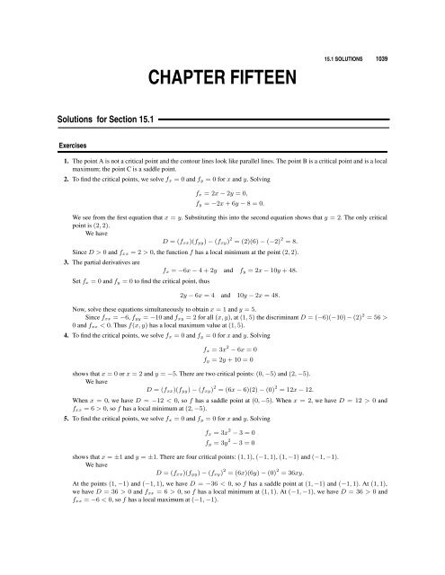
CHAPTER FIFTEEN

CHAPTER FIFTEEN
15.1 SOLUTIONS 1039
Solutions for Section 15.1
Exercises
1. The point A is not a critical point and the contour lines look like parallel lines. The point B is a critical point and is a local
maximum; the point C is a saddle point.
2. To find the critical points, we solve f x = 0 and f y = 0 for x and y. Solving
f x = 2x − 2y = 0,
f y = −2x + 6y − 8 = 0.
We see from the first equation that x = y. Substituting this into the second equation shows that y = 2. The only critical
point is (2, 2).
We have
D = (f xx)(f yy) − (f xy) 2 = (2)(6) − (−2) 2 = 8.
Since D > 0 and f xx = 2 > 0, the function f has a local minimum at the point (2, 2).
3. The partial derivatives are
Set f x = 0 and f y = 0 to find the critical point, thus
f x = −6x − 4 + 2y and f y = 2x − 10y + 48.
2y − 6x = 4 and 10y − 2x = 48.
Now, solve these equations simultaneously to obtain x = 1 and y = 5.
Since f xx = −6, f yy = −10 and f xy = 2 for all (x, y), at (1, 5) the discriminant D = (−6)(−10) − (2) 2 = 56 >
0 and f xx < 0. Thus f(x, y) has a local maximum value at (1, 5).
4. To find the critical points, we solve f x = 0 and f y = 0 for x and y. Solving
f x = 3x 2 − 6x = 0
f y = 2y + 10 = 0
shows that x = 0 or x = 2 and y = −5. There are two critical points: (0, −5) and (2, −5).
We have
D = (f xx)(f yy) − (f xy) 2 = (6x − 6)(2) − (0) 2 = 12x − 12.
When x = 0, we have D = −12 < 0, so f has a saddle point at (0, −5). When x = 2, we have D = 12 > 0 and
f xx = 6 > 0, so f has a local minimum at (2, −5).
5. To find the critical points, we solve f x = 0 and f y = 0 for x and y. Solving
f x = 3x 2 − 3 = 0
f y = 3y 2 − 3 = 0
shows that x = ±1 and y = ±1. There are four critical points: (1, 1), (−1, 1), (1, −1) and (−1, −1).
We have
D = (f xx)(f yy) − (f xy) 2 = (6x)(6y) − (0) 2 = 36xy.
At the points (1, −1) and (−1, 1), we have D = −36 < 0, so f has a saddle point at (1, −1) and (−1, 1). At (1, 1),
we have D = 36 > 0 and f xx = 6 > 0, so f has a local minimum at (1, 1). At (−1, −1), we have D = 36 > 0 and
f xx = −6 < 0, so f has a local maximum at (−1, −1).

1040 Chapter Fifteen /SOLUTIONS
6. To find the critical points, we solve f x = 0 and f y = 0 for x and y. Solving
f x = 3x 2 − 6x = 0
f y = 3y 2 − 3 = 0
shows that x = 0 or x = 2 and y = −1 or y = 1. There are four critical points: (0, −1), (0, 1), (2, −1), and (2, 1).
We have
D = (f xx)(f yy) − (f xy) 2 = (6x − 6)(6y) − (0) 2 = (6x − 6)(6y).
At the point (0, −1), we have D > 0 and f xx < 0, so f has a local maximum.
At the point (0, 1), we have D < 0, so f has a saddle point.
At the point (2, −1), we have D < 0, so f has a saddle point.
At the point (2, 1), we have D > 0 and f xx > 0, so f has a local minimum.
7. To find the critical points, we solve f x = 0 and f y = 0 for x and y. Solving
f x = 3x 2 − 3 = 0
f y = 3y 2 − 12y = 0
shows that x = −1 or x = 1 and y = 0 or y = 4. There are four critical points: (−1, 0), (1, 0), (−1, 4), and (1, 4).
We have
D = (f xx)(f yy) − (f xy) 2 = (6x)(6y − 12) − (0) 2 = (6x)(6y − 12).
At critical point (−1, 0), we have D > 0 and f xx < 0, so f has a local maximum at (−1, 0).
At critical point (1, 0), we have D < 0, so f has a saddle point at (1, 0).
At critical point (−1, 4), we have D < 0, so f has a saddle point at (−1, 4).
At critical point (1, 4), we have D > 0 and f xx > 0, so f has a local minimum at (1, 4).
8. Find the critical point(s) by setting
f x = (xy + 1) + (x + y) · y = y 2 + 2xy + 1 = 0,
f y = (xy + 1) + (x + y) · x = x 2 + 2xy + 1 = 0,
then we get x 2 = y 2 , and so x = y or x = −y.
If x = y, then x 2 + 2x 2 + 1 = 0, that is, 3x 2 = −1, and there is no real solution. If x = −y, then x 2 − 2x 2 + 1 = 0,
which gives x 2 = 1. Solving it we get x = 1 or x = −1, then y = −1 or y = 1, respectively. Hence, (1, −1) and (−1, 1)
are critical points.
Since
f xx(x, y) = 2y,
f xy(x, y) = 2y + 2x
f yy(x, y) = 2x,
and
the discriminant is
D(x, y) = f xxf yy − f 2 xy
= 2y · 2x − (2y + 2x) 2
= −4(x 2 + xy + y 2 ).
thus
Therefore (1, −1) and (−1, 1) are saddle points.
9. At a critical point, f x = 0, f y = 0.
D(1, −1) = −4(1 2 + 1 · (−1) + (−1) 2 ) = −4 < 0,
D(−1, 1) = −4((−1) 2 + (−1) · 1 + 1 2 ) = −4 < 0.
f x = 8y − (x + y) 3 = 0, we know 8y = (x + y) 3 .
f y = 8x − (x + y) 3 = 0, we know 8x = (x + y) 3 .
Therefore we must have x = y. Since (x + y) 3 = (2y) 3 = 8y 3 , this tells us that 8y − 8y 3 = 0. Solving gives y = 0, ±1.
Thus the critical points are (0, 0), (1, 1), (−1, −1).

15.1 SOLUTIONS 1041
f yy = f xx = −3(x + y) 2 , and f xy = 8 − 3(x + y) 2 .
The discriminant is
D(x, y) = f xxf yy − f 2 xy
= 9(x + y) 4 − ( 64 − 48(x + y) 2 + 9(x + y) 4)
= −64 + 48(x + y) 2 .
D(0, 0) = −64 < 0, so (0, 0) is a saddle point.
D(1, 1) = −64 + 192 > 0 and f xx(1, 1) = −12 < 0, so (1, 1) is a local maximum.
D(−1, −1) = −64 + 192 > 0 and f xx(−1, −1) = −12 < 0, so (−1, −1) is a local maximum.
10. To find the critical points, we solve f x = 0 and f y = 0 for x and y. Solving
f x = 6 − 2x + y = 0,
f y = x − 2y = 0.
We see from the second equation that x = 2y. Substituting this into the first equation shows that y = 2. The only critical
point is (4, 2).
We have
D = (f xx)(f yy) − (f xy) 2 = (−2)(−2) − 1 2 = 3.
Since D > 0 and f xx = −2 < 0, the function f has a local maximum at (4, 2).
11. To find the critical points, we solve f x = 0 and f y = 0 for x and y. Solving
shows that the only critical point is (0, 0).
We have
f x = e 2x2 +y 2 (4x) = 0,
f y = e 2x2 +y 2 (2y) = 0,
D = (f xx)(f yy) − (f xy) 2 = e 2x2 +y 2 (4 + (4x) 2 ) · e 2x2 +y 2 (2 + (2y) 2 ) − (e 2x2 +y 2 (4x · 2y)) 2 .
At (0, 0), we have D = 4 · 2 − 0 2 > 0 and f xx = 4 > 0, so the function has a local minimum at the point (0, 0).
12. At the origin f(0, 0) = 0. Since x 6 ≥ 0 and y 6 ≥ 0, the point (0, 0) is a local (and global) minimum. The second
derivative test does not tell you anything since D = 0.
13. At the origin g(0, 0) = 0. Since y 3 ≥ 0 for y > 0 and y 3 < 0 for y < 0, the function g takes on both positive and negative
values near the origin, which must therefore be a saddle point. The second derivative test does not tell you anything since
D = 0.
14. At the origin h(0, 0) = 1. Since cos x and cos y are never above 1, the origin must be a local (and global) maximum. The
second derivative test
D = h xxh yy − (h xy) 2 = ( (− cos x cos y)(− cos x cos y) − (sin x sin y) 2) ∣ ∣
x=0,y=0
= ( cos 2 x cos 2 y − sin 2 x sin 2 y ) ∣ ∣
x=0,y=0
= 1 > 0
and h xx(0, 0) < 0, so (0, 0) is a local maximum.
15. At the origin, the second derivative test gives
Thus k(0, 0) is a saddle point.
D = k xxk yy − (k xy) 2 = ( (− sin x sin y)(− sin x sin y) − (cos x cos y) 2)∣ ∣
x=0,y=0
= sin 2 0 sin 2 0 − cos 2 0 cos 2 0
= −1 < 0.
Problems
16. (a) P is a local maximum.
(b) Q is a saddle point.
(c) R is a local minimum.
(d) S is none of these.

1042 Chapter Fifteen /SOLUTIONS
17. Figure 15.1 shows the gradient vectors around P and Q pointing perpendicular to the contours and in the direction of
increasing values of the function.
y
−2
5
3
1
S
1
6
2
4
−1
−3
−6
−5
−4
−1
✒✿
R
✙ ■ 3
☛ ❘
❲
0 0
✒✒ ■ Q
❘❘ ✠ ❨ ✐✛
✮ ✙
0 0
−6
−5
−4
−6
x
−3
−1
2
4
❘ P
✶
✲ ✠
✐
✛
6
5
3
1
−2
6
Figure 15.1
18. Figure 15.2 shows the direction of ∇f at the points where ‖∇f‖ is largest, since at those points the contours are closest
together.
y
−6
−5
−4
−2
3
1
S
5
✠ R
−1
0 0
0 0
4
2
1
Q
−1
−3
−5
−6
−6
−4
x
−3
−1
P
−2
2
4
6
5
6
3
1
Figure 15.2
19. First, we identify the critical points. The partials are f x(x, y) = 3x 2 and f y(x, y) = −2ye −y2 . These will vanish
simultaneously when x = 0 and y = 0, so our only critical point is (0, 0). The discriminant is
D = f xx(x, y)f yy(x, y) − f 2 xy(x, y) = (6x)(4y 2 e −y2 − 2e −y2 ) − 0 = 12xe −y2 (2y 2 − 1).
Unfortunately, the discriminant is zero at the origin so the second derivative test can tell us nothing about our critical point.
We can, however, see that we are at a saddle point by looking at the behavior of f(x, y) along the line y = 0. Here we have
f(x, 0) = x 3 + 1, so for positive x, we have f(x, 0) > 1 = f(0, 0) and for negative x, we have f(x, 0) < 1 = f(0, 0).
So f(x, y) has neither a maximum nor a minimum at (0, 0).

15.1 SOLUTIONS 1043
20. To find critical points, set partial derivatives equal to zero:
The critical points are
To classify, calculate D = E xxE yy − (E xy) 2 = cos x.
At the points (0, 0), (±2π, 0), (±4π, 0), (±6π, 0), · · ·
E x = sin x = 0 when x = 0, ±π, ±2π, · · ·
E y = y = 0 when y = 0.
· · · (−2π, 0), (−π, 0), (0, 0), (π, 0), (2π, 0), (3π, 0) · · ·
D = (1) > 0 and E xx > 0 (SinceE xx(0, 2kπ) = cos(2kπ) = 1).
Therefore (0, 0), (±2π, 0), (±4π, 0), (±6π, 0), · · · are local minima.
At the points (±π, 0), (±3π, 0), (±5π, 0), (±7π, 0), · · ·, we have cos(2k + 1)π = −1, so
D = (−1) < 0.
Therefore (±π, 0), (±3π, 0), (±5π, 0), (±7π, 0), · · · are saddle points.
21. To find the critical points, we must solve the equations
The first equation has solution
The second equation has solution
Since x can be anything, the lines
are lines of critical points.
We calculate
∂f
∂x = ex (1 − cos y) = 0
∂f
∂y = ex (sin y) = 0.
y = 0, ±2π, ±4π, . . . .
y = 0, ±π, ±2π, ±3π, . . . .
y = 0, ±2π, ±4π, . . .
D = (f xx)(f yy) − (f xy) 2 = e x (1 − cos y)e x cos y − (e x sin y) 2
= e 2x (cos y − cos 2 y − sin 2 y)
= e 2x (cos y − 1)
At any critical point on one of the lines y = 0, y = ±2π, y = ±4π, . . .,
D = e 2x (1 − 1) = 0.
Thus, D tells us nothing. However, all along these critical lines, the value of the function, f, is zero. Since the function f
is never negative, the critical points are all both local and global minima.
22. At a critical point,
and
f x = cos x sin y = 0 so cos x = 0 or sin y = 0;
Case 1: Assume cos x = 0. This gives
f y = sin x cos y = 0 so sin x = 0 or cos y = 0.
x = · · · − 3π 2 , − π 2 , π 2 , 3π 2 , · · ·
(This can be written more compactly as: x = kπ + π/2, for k = 0, ±1, ±2, · · ·.)
If cos x = 0, then sin x = ±1 ≠ 0. Thus in order to have f y = 0 we need cos y = 0, giving
y = · · · − 3π 2 , − π 2 , π 2 , 3π 2 , · · ·

1044 Chapter Fifteen /SOLUTIONS
(More compactly, y = lπ + π/2, for l = 0, ±1, ±2, · · ·)
Case 2: Assume sin y = 0. This gives
y = · · · − 2π, −π, 0, π, 2π, · · ·
(More compactly, y = lπ, for l = 0, ±1, ±2, · · ·)
If sin y = 0, then cos y = ±1 ≠ 0, so to get f y = 0 we need sin x = 0, giving
x = · · · , −2π, −π, 0, π, 2π, · · ·
(More compactly, x = kπ for k = 0, ±0, ±1, ±2, · · ·)
Hence we get all the critical points of f(x, y). Those from Case 1 are as follows:
(
· · · − π 2 , − π ) (
, − π 2 2 , π ) (
, − π 2 2 , 3π 2
Those from Case 2 are as follows:
· · ·
More compactly these points can be written as,
( π
· · ·
2 , − π )
2
( 3π
2 , − π 2
)
,
( π
,
2 , π )
2
( 3π
2 , π 2
)
,
( π
,
2 , 3π )
2
( 3π
2 , 3π 2
)
· · ·
· · ·
)
· · ·
· · · (−π, −π), (−π, 0), (−π, π), (−π, 2π) · · ·
· · · (0, −π), (0, 0), (0, π), (0, 2π) · · ·
· · · (π, −π), (π, 0), (π, π), (π, 2π) · · ·
(kπ, lπ), for k = 0, ±1, ±2, · · · , l = 0, ±1, ±2, · · ·
and (kπ + π 2 , lπ + π ), for k = 0, ±1, ±2, · · · , l = 0, ±1, ±2, · · ·
2
To classify the critical points, we find the discriminant. We have
f xx = − sin x sin y, f yy = − sin x sin y, and f xy = cos x cos y.
Thus the discriminant is
D(x, y) = f xxf yy − f 2 xy
= (− sin x sin y)(− sin x sin y) − (cos x cos y) 2
= sin 2 x sin 2 y − cos 2 x cos 2 y
= sin 2 y − cos 2 x. (Use: sin 2 x = 1 − cos 2 x and factor.)
At points of the form (kπ, lπ) where k = 0, ±1, ±2, · · · ; l = 0, ±1, ±2, · · ·, we have
D(x, y) = −1 < 0 so (kπ, lπ) are saddle points.
At points of the form (kπ + π , lπ + π ) where k = 0, ±1, ±2, · · · ; l = 0, ±1, ±2, · · ·
2 2
D(kπ + π , lπ + π ) = 1 > 0, so we have two cases:
2 2
If k and l are both even or k and l are both odd, then
f xx = − sin x sin y = −1 < 0, so (kπ + π , lπ + π ) are local maximum points.
2 2
If k is even but l is odd or k is odd but l is even, then
f xx = 1 > 0 so (kπ + π , lπ + π ) are local minimum points.
2 2
23. At a local maximum value of f,
∂ f
= −2x − B = 0.
∂ x
We are told that this is satisfied by x = −2. So −2(−2) − B = 0 and B = 4. In addition,
∂ f
∂ y = −2y − C = 0
and we know this holds for y = 1, so −2(1) − C = 0, giving C = −2. We are also told that the value of f is 15 at the
point (−2, 1), so
15 = f(−2, 1) = A − ((−2) 2 + 4(−2) + 1 2 − 2(1)) = A − (−5), so A = 10.

and
15.1 SOLUTIONS 1045
Now we check that these values of A, B, and C give f(x, y) a local maximum at the point (−2, 1). Since
f xx(−2, 1) = −2,
f yy(−2, 1) = −2
f xy(−2, 1) = 0,
we have that f xx(−2, 1)f yy(−2, 1) − f 2 xy(−2, 1) = (−2)(−2) − 0 > 0 and f xx(−2, 1) < 0. Thus, f has a local
maximum value 15 at (−2, 1).
24. (a) (1, 3) is a critical point. Since f xx > 0 and the discriminant
the point (1, 3) is a minimum.
(b) See Figure 15.3.
D = f xxf yy − f 2 xy = f xxf yy − 0 2 = f xxf yy > 0,
y
0
y
120
64
32
16
4
1
3
1
✠
x
−7
−5
1
−3
0
1
1
3 579
−1
0
1
0
0
5 79
3
−1
−3
−5
−7
x
Figure 15.3
Figure 15.4
25. (a) (a, b) is a critical point. Since the discriminant D = f xxf yy − f 2 xy = −f 2 xy < 0, (a, b) is a saddle point.
(b) See Figure 15.4.
26. Begin by constructing little pieces of the contour diagram around each of the points (−1, 0), (3, 3), and (3, −3) where
some information about f is given. The general shape will be as in Figure 15.5, and the directions of increasing contour
values are indicated for each part. Then complete the diagram in any way. One possible solution is given in Figure 15.6.
0 1
2
0 1 2
3
4
Figure 15.5: Part of contour
diagram with arrows showing
direction of increasing
function values
Figure 15.6: Contour diagram
of f(x, y)

1046 Chapter Fifteen /SOLUTIONS
27. Since (2, 4) is a local minimum, the contours around (2, 4) are closed curves with increasing values as we go away from
the point (2, 4). We assume that the function values continue to increase as we move parallel to the y-axis to the point
(2, 1). Since (2, 1) is a saddle point, we draw the contours so that the values go down as we move up or down from this
point, and up as we move to the left or right. One possible contour diagram is shown in Figure 15.7.
y
y
6
5
f = −1
4
3
2
1
−4
−3
−2
−1
0 1 2 3 4
f = 1
(0, 0)
f = 1
f = 0
f = 0
x
−1
−1 1 2 3 4 5 6
−1
x
f = −1
Figure 15.7
Figure 15.8
28. (a) Setting the partial derivatives equal to 0, we have
f x(x, y) = 2x(x 2 + y) + 2x(x 2 − y) = 4x 3 = 0
f y(x, y) = −(x 2 + y) + (x 2 − y) = −2y = 0.
Thus, (0, 0) is the only critical point.
(b) Calculating D gives
D = (f xx)(f yy) − (f xy) 2 = (12x 2 )(−2) − 0 2 = −24x 2 .
At x = 0, y = 0, we have
D(0, 0) = 0.
Thus the second derivative test tells us nothing about the nature of the critical point.
(c) Since f(0, 0) = 0, we sketch contours with values near 0. The contour f = 0 is given by
that is, the two parabolas
(x 2 − y)(x 2 + y) = 0,
y = x 2 and y = −x 2
We also sketch the contours f = 1 and f = −1. See Figure 15.8.
Since there are values of the function which are both positive (above f(0, 0)) and negative (below (f(0, 0)),
near the critical point (0, 0), the origin is neither a local maximum nor a local minimum; it is a saddle point.
29. We have f x = 2kx − 4y and f y = 2y − 4x, so f xx = 2k, f xy = −4, and f yy = 2. The discriminant is
D = (f xx)(f yy) − (f xy) 2 = (2k)(2) − (−4) 2 = 4k − 16.
Since D = 4k − 16, we see that D < 0 when k < 4. The function has a saddle point at the point (0, 0) when k < 4.
When k > 4, we have D > 0 and f xx > 0, so the function has a local minimum at the point (0, 0). When k = 4,
the discriminant is zero, and we get no information about this critical point. By looking at the values of the function in
Table 15.1, it appears that f has a local minimum at the point (0, 0) when k = 4.
Table 15.1
y
−0.1 0 0.1
−0.1 0.01 0.01 0.09
0 0.04 0 0.04
0.1 0.09 0.01 0.01
x
(a) The function f(x, y) has a saddle point at (0, 0) if k < 4.

15.1 SOLUTIONS 1047
(b) There are no values of k for which this function has a local maximum at the point (0, 0).
(c) The function f(x, y) has a local minimum at (0, 0) if k ≥ 4.
30. The first order partial derivatives are
And the second order partial derivatives are
f x(x, y) = 2kx − 2y and f y(x, y) = 2ky − 2x.
f xx(x, y) = 2k f xy(x, y) = −2 f yy(x, y) = 2k
Since f x(0, 0) = f y(0, 0) = 0, the point (0, 0) is a critical point. The discriminant is
D = (2k)(2k) − 4 = 4(k 2 − 1).
For k = ±2, the discriminant is positive, D = 12. When k = 2, f xx(0, 0) = 4 which is positive so we have a local
minimum at the origin. When k = −2, f xx(0, 0) = −4 so we have a local maximum at the origin. In the case k = 0,
D = −4 so the origin is a saddle point.
Lastly, when k = ±1 the discriminant is zero, so the second derivative test can tell us nothing. Luckily, we can factor
f(x, y) when k = ±1. When k = 1,
f(x, y) = x 2 − 2xy + y 2 = (x − y) 2 .
This is always greater than or equal to zero. So f(0, 0) = 0 is a minimum and the surface is a trough-shaped parabolic
cylinder with its base along the line x = y.
When k = −1,
f(x, y) = −x 2 − 2xy − y 2 = −(x + y) 2 .
This is always less than or equal to zero. So f(0, 0) = 0 is a maximum. The surface is a parabolic cylinder, with its top
ridge along the line x = −y.
k = −2
y
k = −1
y k = 0
y
−16
−12
−8
−4
−1
x
−1
−5
−10
−20
−30
−30
−20
−10
−5
−1
x
16
12
8
4
1
−1
−4
−8
−12
−16
−1
1
−4
4
−16
−12
−8
8
12
16
x
k = 1
y
k = 2
y
30
20
10
5
1
1
x
1
4
8
16
12
x
5
10
20
30
Figure 15.9

1048 Chapter Fifteen /SOLUTIONS
31. The partial derivatives are
f x(x, y) = 3x 2 − 3y 2 and f y(x, y) = −6xy.
Now f x(x, y) will vanish if x = ±y and f y(x, y) will vanish if either x = 0 or y = 0. Since the partial derivatives
are defined everywhere, the only critical points are where f x(x, y) and f y(x, y) vanish simultaneously. (0, 0) is the only
critical point.
To find the contour for f(x, y) = 0, we solve the equation x 3 − 3xy 2 = 0. This can be factored into
f(x, y) = x(x − √ 3 y)(x + √ 3 y) = 0
whose roots are x = 0, x = √ 3 y and x = − √ 3 y. Each of these roots describes a line through the origin; the three of
them divide the plane into six regions. Crossing any one of these lines will change the sign of only one of the three factors
of f(x, y), which will change the sign of f(x, y).
y
f > 0
f < 0
2
11
−1
−2
✛ y = x
√
3
−2
f < 0
0
−1
0 0
1 2
0 0
f > 0
x
2
11
−1
−2
✛ y = −x
√
3
f > 0 f < 0
Figure 15.10
Solutions for Section 15.2
Exercises
1. Mississippi lies entirely within a region designated as 80s so we expect both the maximum and minimum daily high
temperatures within the state to be in the 80s. The southwestern-most corner of the state is close to a region designated as
90s, so we would expect the temperature here to be in the high 80s, say 87-88. The northern-most portion of the state is
located near the center of the 80s region. We might expect the high temperature there to be between 83-87.
Alabama also lies completely within a region designated as 80s so both the high and low daily high temperatures
within the state are in the 80s. The southeastern tip of the state is close to a 90s region so we would expect the temperature
here to be about 88-89 degrees. The northern-most part of the state is near the center of the 80s region so the temperature
there is 83-87 degrees.
Pennsylvania is also in the 80s region, but it is touched by the boundary line between the 80s and a 70s region. Thus
we expect the low daily high temperature to occur there and be about 80 degrees. The state is also touched by a boundary
line of a 90s region so the high will occur there and be 89-90 degrees.
New York is split by a boundary between an 80s and a 70s region, so the northern portion of the state is likely to be
about 74-76 while the southern portion is likely to be in the low 80s, maybe 81-84 or so.
California contains many different zones. The northern coastal areas will probably have the daily high as low as
65-68, although without another contour on that side, it is difficult to judge how quickly the temperature is dropping off
to the west. The tip of Southern California is in a 100s region, so there we expect the daily high to be 100-101.
Arizona will have a low daily high around 85-87 in the northwest corner and a high in the 100s, perhaps 102-107 in
its southern regions.
Massachusetts will probably have a high daily high around 81-84 and a low daily high of 70.

15.2 SOLUTIONS 1049
2. Let the line be in the form y = b + mx. When x equals −1, 0 and 1, then y equals b − m, b, and b + m, respectively. The
sum of the squares of the vertical distances, which is what we want to minimize, is
f(m, b) = (2 − (b − m)) 2 + (−1 − b) 2 + (1 − (b + m)) 2 .
To find the critical points, we compute the partial derivatives with respect to m and b,
f m = 2(2 − b + m) + 0 + 2(1 − b − m)(−1)
= 4 − 2b + 2m − 2 + 2b + 2m
= 2 + 4m,
f b = 2(2 − b + m)(−1) + 2(−1 − b)(−1) + 2(1 − b − m)(−1)
= −4 + 2b − 2m + 2 + 2b − 2 + 2b + 2m
= −4 + 6b.
Setting both partial derivatives equal to zero, we get a system of equations:
2 + 4m = 0,
−4 + 6b = 0.
The solution is m = −1/2 and b = 2/3. One can check that it is a minimum. Hence, the regression line is y = 2 3 − 1 2 x.
3. The function f has no global maximum or global minimum.
4. The function g has a global minimum (it is 0) but no global maximum.
5. The function h has no global maximum or minimum.
6. Since f(x, y) ≤ 0 for all x, y and sincef(0, 0) = 0, the function has a global maximum (it is 0) and no global minimum.
7. Suppose x is fixed. Then for large values of y the sign of f is determined by the highest power of y, namely y 3 . Thus,
So f does not have a global maximum or minimum.
f(x, y) → ∞ as y → ∞
f(x, y) → −∞ as y → −∞.
8. To maximize z = x 2 + y 2 , it suffices to maximize x 2 and y 2 . We can maximize both of these at the same time by
taking the point (1, 1), where z = 2. It occurs on the boundary of the square. (Note: We also have maxima at the points
(−1, −1), (−1, 1) and (1, −1) which are on the boundary of the square.)
To minimize z = x 2 + y 2 , we choose the point (0, 0), where z = 0. It does not occur on the boundary of the square.
9. To maximize z = −x 2 − y 2 it suffices to minimize x 2 and y 2 . Thus, the maximum is at (0, 0), where z = 0. It does not
occur on the boundary of the square.
To minimize z = −x 2 − y 2 , it suffices to maximize x 2 and y 2 . Do this by taking the point (1, 1), (−1, −1), (−1, 1),
or (1, −1) where z = −2. These occur on the boundary of the square.
10. To maximize this function, it suffices to maximize x 2 and minimize y 2 . We can do this by choosing the point (1, 0), or
(−1, 0) where z = 1. These occur on the boundary of the square.
To minimize z = x 2 − y 2 , it suffices to maximize y 2 and minimize x 2 . We can do this by taking the point (0, 1), or
(0, −1) where z = −1. These occur on the boundary of the square.
11. The maximum value, which is slightly above 30, say 30.5, occurs approximately at the origin. The minimum value, which
is about 20.5, occurs at (2.5, 5).
12. The maxima occur at about (π/2, 0) and (π/2, 2π). The minimum occurs at (π/2, π). The maximum value is about 1,
the minimum value is about −1.
13. The maximum value, which is about 11, occurs at (5.1, 4.9). The minimum value, which is about −1, occurs at (1, 3.9).
Problems
14. To find critical points of g we solve
g x(x, y) = Ax + By − D = 0
g y(x, y) = Bx + Cy − E = 0

1050 Chapter Fifteen /SOLUTIONS
which is equivalent to
Ax + By = D
Bx + Cy = E.
The second derivative test shows that the critical point gives a minimum for g because g xxg yy − g 2 xy = AC − B 2 > 0
and g xx = A > 0.
15. The variables are a and b, so we set
so, collecting terms and dividing by 4 and 2 respectively,
∂S
= 2(a + b) + 8(4a + b − 2) + 18(9a + b − 4) = 0
∂a
∂S
= 2(a + b) + 2(4a + b − 2) + 2(9a + b − 4) = 0,
∂b
49a + 7b − 22 = 0
14a + 3b − 6 = 0.
Solving gives a = 24/49, b = −2/7.
Since there is only one critical point and S is unbounded as a, b → ∞, this critical point is the global minimum.
Therefore, the best fitting parabola is
y = 24
49 x2 − 2 7 .
16. We must find b and m to minimize the function
g(b, m) =
=
∫ 1
0
∫ 1
0
(x 2 − (b + mx)) 2 dx
(x 4 − 2bx 2 + b 2 − 2mx 3 + 2bmx + m 2 x 2 )dx
= 1 5 − 2 3 b + b2 − m 2
The critical points of g are given by the equations
+ bm +
m2
3 .
∂g
∂b = − 2 3 + 2b + m = 0
∂g
∂m = − 1 2 + b + 2 3 m = 0.
The solution is b = −1/6 and m = 1. The linear least squares approximation of x 2 on the interval [0, 1] is L(x, y) =
−1/6 + x.
17. We must find b and m to minimize the function
g(b, m) =
=
∫ 1
0
∫ 1
0
(x 3 − (b + mx)) 2 dx
(x 6 − 2bx 3 + b 2 − 2mx 4 + 2bmx + m 2 x 2 )dx
= 1 6 − 1 2 b + b2 − 2m 5
The critical points of g are given by the equations
+ bm +
m2
3 .
∂g
∂b = − 1 2 + 2b + m = 0
∂g
∂m = − 2 5 + b + 2 3 m = 0.
The solution is b = −1/5 and m = 9/10. The linear least squares approximation of x 3 on the interval [0, 1] is L(x, y) =
−0.2 + 0.9x.

15.2 SOLUTIONS 1051
18. We calculate the partial derivatives and set them to zero.
∂ (range)
∂t
∂ (range)
∂h
= −10t − 6h + 400 = 0
= −6t − 6h + 300 = 0.
solving we obtain
so
10t + 6h = 400
6t + 6h = 300
4t = 100
t = 25
Solving for h, we obtain 6h = 150, yielding h = 25. Since the range is quadratic in h and t, the second derivative test
tells us this is a local and global maximum. So the optimal conditions are h = 25% humidity and t = 25 ◦ C.
19. (a) This tells us that an increase in the price of either product causes a decrease in the quantity demanded of both
products. An example of products with this relationship is tennis rackets and tennis balls. An increase in the price of
either product is likely to lead to a decrease in the quantity demanded of both products as they are used together. In
economics, it is rare for the quantity demanded of a product to increase if its price increases, so for q 1, the coefficient
of p 1 is negative as expected. The coefficient of p 2 in the expression could be either negative or positive. In this case,
it is negative showing that the two products are complementary in use. If it were positive, however, it would indicate
that the two products are competitive in use, for example Coke and Pepsi.
(b) The revenue from the first product would be q 1p 1 = 150p 1 − 2p 2 1 − p 1p 2, and the revenue from the second product
would be q 2p 2 = 200p 2 − p 1p 2 − 3p 2 2. The total sales revenue of both products, R, would be
R(p 1, p 2) = 150p 1 + 200p 2 − 2p 1p 2 − 2p 2 1 − 3p 2 2.
Note that R is a function of p 1 and p 2. To find the critical points of R, set ∇R = 0, i.e.,
This gives
and
∂R
∂p 1
= ∂R
∂p 2
= 0.
∂R
∂p 1
= 150 − 2p 2 − 4p 1 = 0
∂R
∂p 2
= 200 − 2p 1 − 6p 2 = 0
Solving simultaneously, we have p 1 = 25 and p 2 = 25. Therefore the point (25, 25) is a critical point for R. Further,
∂ 2 R
∂p 2 1
so the discriminant at this critical point is
= −4, ∂2 R
∂p 2 2
= −6,
∂ 2 R
∂p 1∂p 2
= −2,
D = (−4)(−6) − (−2) 2 = 20.
Since D > 0 and ∂ 2 R/∂p 2 1 < 0, this critical point is a local maximum. Since R is quadratic in p 1 and p 2, this is a
global maximum. Therefore the maximum possible revenue is
R = 150(25) + 200(25) − 2(25)(25) − 2(25) 2 − 3(25) 2
= (6)(25) 2 + 8(25) 2 − 7(25) 2
= 4375.
This is obtained when p 1 = p 2 = 25. Note that at these prices, q 1 = 75 units, and q 2 = 100 units.

1052 Chapter Fifteen /SOLUTIONS
20. The total revenue is
and as q = q 1 + q 2, this gives
R = pq = (60 − 0.04q)q = 60q − 0.04q 2 ,
R = 60q 1 + 60q 2 − 0.04q 2 1 − 0.08q 1q 2 − 0.04q 2 2.
Therefore, the profit is
P (q 1, q 2) = R − C 1 − C 2
At a local maximum point, we have grad P = ⃗0 :
Solving these equations, we find that
= −13.7 + 60q 1 + 60q 2 − 0.07q 2 1 − 0.08q 2 2 − 0.08q 1q 2.
∂P
∂q 1
= 60 − 0.14q 1 − 0.08q 2 = 0,
∂P
∂q 2
= 60 − 0.16q 2 − 0.08q 1 = 0.
q 1 = 300 and q 2 = 225.
To see whether or not we have found a local maximum, we compute the second-order partial derivatives:
Therefore,
∂ 2 P
∂q 2 1
D = ∂2 P
∂q 2 1
= −0.14,
∂ 2 P
∂q 2 2
−
∂ 2 P
∂q 2 2
= −0.16,
∂ 2 P
∂q 1∂q 2
= −0.08.
∂2 P
∂q 1∂q 2
= (−0.14)(−0.16) − (−0.08) 2 = 0.016,
and so we have found a local maximum point. The graph of P (q 1, q 2) has the shape of an upside down paraboloid since
P is quadratic in q 1 and q 2, hence (300, 225) is a global maximum point.
21. (a) The revenue R = p 1q 1 + p 2q 2. Profit = P = R − C = p 1q 1 + p 2q 2 − 2q 2 1 − 2q 2 2 − 10.
∂P
= p 1 − 4q 1 = 0
∂q 1
∂P
= p 2 − 4q 2 = 0
∂q 2
gives q 1 = p1
4
gives q 2 = p2
4
Since ∂2 P
∂q 2 1
and ∂2 P
∂q 2 1
= −4, ∂2 P
= −4 and ∂2 P
∂q
2
2 ∂q 1 ∂q 2
= 0, at (p 1/4, p 2/4) we have that the discriminant, D = (−4)(−4) > 0
< 0, thus P has a local maximum value at (q 1, q 2) = (p 1/4, p 2/4). Since P is quadratic in q 1 and q 2, this
is a global maximum. So P = p2 1
4
+ p2 2
4
− 2 p2 1
16 − 2 p2 2
16 − 10 = p2 1
8
+ p2 2
8
− 10 is the maximum profit.
(b) The rate of change of the maximum profit as p 1 increases is
∂
∂p 1
(max P ) = 2p1
8 = p1
4 .
22. We want to maximize the theater’s profit, P , as a function of the two variables (prices) p c and p a. As always, P = R − C,
where R is the revenue, R = q cp c + q ap a, and C is the cost, which is of the form C = k(q c + q a) for some constant k.
Thus,
P (p c, p a) = q cp c + q ap a − k(q c + q a)
= rp −3
c
− krp −4
c
+ sp −1
a
− ksp −2
a
To find the critical points, solve
We get p c = 4k/3 and p a = 2k.
∂P
= −3rp −4
c + 4krp −5
c = 0
∂p c
∂P
= −sp −2
a + 2ksp −3
a = 0.
∂p a

15.2 SOLUTIONS 1053
This critical point is a global maximum by the following useful, general argument. Suppose that F (x, y) = f(x) +
g(y), where f has a global maximum at x = b and g has a global maximum at y = d. Then for all x, y:
so F has global maximum at x = b, y = d.
The profit function in this problem has the form
F (x, y) = f(x) + g(y) ≤ f(b) + g(d) = F (b, d),
P (p c, p a) = f(p c) + g(p a),
and the usual single-variable calculus argument using f ′ and g ′ shows that p c = 4k/3 and p a = 2k are global maxima
for f and g, respectively. Thus the maximum profit occurs when p c = 4k/3 and p a = 2k. Thus,
p c
= 4k/3
p a 2k = 2 3 .
23. Let the sides be x, y, z cm. Then the volume is given by V = xyz = 32.
The surface area S is given by
S = 2xy + 2xz + 2yz.
Substituting z = 32/(xy) gives
At a critical point,
S = 2xy + 64
y + 64 x .
∂S
∂x
∂S
∂y
= 2y −
64
x 2 = 0
= 2x −
64
y 2 = 0,
The symmetry of the equations (or by dividing the equations) tells us that x = y and
2x − 64
x 2 = 0
x 3 = 32
x = 32 1/3 = 3.17 cm.
Thus the only critical point is x = y = (32) 1/3 cm and z = 32/ ( (32) 1/3 · (32) 1/3) = (32) 1/3 cm. At the critical point
S xxS yy − (S xy) 2 = 128
x 3 · 128
y 3 − 22 = (128)2
x 3 y 3 − 4.
Since D > 0 and S xx > 0 at this critical point, the critical point x = y = z = (32) 1/3 is a local minimum. Since
S → ∞ as x, y → ∞, the local minimum is a global minimum.
24. Let the sides of the base be x and y cm. Let the height be z cm. Then the volume is given by xyz = 32 and the surface
area, S, is given by
S = xy + 2xz + 2yz.
Substituting z = 32/(xy) gives
At a critical point
The symmetry of the equations tells us that x = y and
S = xy + 64
y + 64 x .
∂S
∂x = y − 64
x = 0 2
∂S
∂y = x − 64
y = 0. 2
x − 64
x 2 = 0
x 3 = 64
x = 4 cm.

1054 Chapter Fifteen /SOLUTIONS
Thus the only critical point is x = y = 4 cm and z = 32/(4 · 4) = 2 cm. At the critical point
D = S xxS yy − (S xy) 2 = 128
x 3 · 128
y 3 − 12 = (128)2
x 3 y 3 − 1.
Since D > 0 and S xx > 0 at this critical point, the critical point x = y = 4, z = 2 is a local minimum. Since S → ∞ as
x, y → ∞, the local minimum is a global minimum.
25. If the coordinates of the corner on the plane are (x, y, z), the volume of the box is V = xyz. Since z = 1 − 3x − 2y on
the plane, the volume is given by
26.
V = xy(1 − 3x − 2y) = xy − 3x 2 y − 2xy 2 .
The domain is the triangular region 0 ≤ x ≤ 1 , 0 ≤ y ≤ (1 − 3x)/2. At a critical point,
3
∂V
∂x = y − 6xy − 2y2 = y(1 − 6x − 2y) = 0
∂V
∂y = x − 3x2 − 4xy = x(1 − 3x − 4y) = 0,
One solution is x = y = 0. Another is x = 0, y = 1 ; another is y = 0, x = 1 . Another is the solution of
2 3
1 − 6x − 2y = 0
1 − 3x − 4y = 0,
namely x = 1 9 , y = 1 6 .
If either x = 0 or y = 0, then V = 0, so these solutions do not give the maximum volume. Since
D = V xxV yy − (V xy) 2 = (−6y)(−4x) − (1 − 6x − 4y) 2
( 1
D
9 , 1 (
= −6 ·
6) 1
6
) (
−4 · 1 ) (
− 1 − 6 · 1
9
9 − 4 · 1 ) 2
= 4 6 9 − 1 9 = 1 3 > 0,
and V xx( 1 9 , 1 6 ) = −1 < 0, the point x = 1 9 , y = 1 6 , is a local maximum at which V = (1/9)(1/6) − 3(1/9)2 (1/6) −
2(1/9)(1/6) 2 = 1/162.
Since all points on the boundary of the domain give V = 0, the local maximum is a global maximum.
h
w
Figure 15.11
l
Let w, h and l be width, height and length of the suitcase in cm. Then its volume V = lwh, and w + h + l ≤ 135.
To maximize the volume V , choose w + h + l = 135, and thus l = 135 − w − h,
Differentiating gives
Find the critical points by solving V w = 0 and V h = 0:
V = wh(135 − w − h)
= 135wh − w 2 h − wh 2
V w = 135h − 2wh − h 2 ,
V h = 135w − w 2 − 2wh.
V w = 0 gives 135h − h 2 = 2wh,
V h = 0 gives 135w − w 2 = 2wh.

15.2 SOLUTIONS 1055
As hw ≠ 0, we cancel h (and w respectively) in the above equations and get
135 − h = 2w
135 − w = 2h
27.
Subtracting gives
w − h = 2(w − h)
hence w = h. Therefore, substituting into the equation V w = 0
and therefore
Since h ≠ 0, we have
135h − h 2 = 2h 2
3h 2 = 135h.
h = 135
3 = 45.
So w = h = 45 cm. Thus, l = 135 − w − h = 45 cm. To check that this critical point is a maximum, we find
so
V ww = −2h,
V hh = −2w,
V wh = 135 − 2w − 2h,
D = V wwV hh − V 2 wh = 4hw − (135 − 2w − 2h) 2 .
At w = h = 45, we have V ww = −2(45) < 0 and D = 4(45) 2 − (135 − 90 − 90) 2 = 6075 > 0, hence V is maximum
at w = h = l = 45.
Therefore, the suitcase with maximum volume is a cube with dimensions width = height = length = 45 cm.
h
w
l
Figure 15.12
The box is shown in Figure 15.12. Cost of four sides = (2hl + 2wh)(1)c/. Cost of two bottoms = (2wl)(2)c/. Thus
the total cost C (in cents) of the box is
C = 2(hl + wh) + 4wl.
But volume wlh = 512, so l = 512/(wh), thus
C = 1024
w
To minimize C, find the critical points of C by solving
We get
+ 2wh +
2048
h .
C h = 2w − 2048
h 2 = 0,
C w = 2h − 1024
w 2 = 0.
2wh 2 = 2048
2hw 2 = 1024.

1056 Chapter Fifteen /SOLUTIONS
Since w, h ≠ 0, we can divide the first equation by the second giving
so
thus
2wh 2
2hw 2 = 2048
1024 ,
h
w = 2,
h = 2w.
Substituting this in C h = 0, we obtain h 3 = 2048, so h = 12.7 cm. Thus w = h/2 = 6.35 cm, and l = 512/(wh) =
6.35 cm. Now we check that these dimensions minimize the cost C. We find that
D = C hh C ww − Chw 2 = ( 4096 2048
)(
h3 w ) − 3 22 ,
and at h = 12.7, w = 6.35, C hh > 0 and D = 16 − 4 > 0, thus C has a local minimum at h = 12.7 and w = 6.35.
Since C increases without bound as w, h → 0 or ∞, this local minimum must be a global minimum.
Therefore, the dimensions of the box that minimize the cost are w = 6.35 cm, l = 6.35 cm and h = 12.7 cm.
28. The square of the distance from the point (x, y, z) to the origin is
If the point is on the plane, z = 1 − 3x − 2y, we have
At the critical point
Simplifying gives
S = x 2 + y 2 + z 2 .
S = x 2 + y 2 + (1 − 3x − 2y) 2 .
∂S
= 2x + 2(1 − 3x − 2y)(−3) = 2(10x + 6y − 3) = 0
∂x
∂S
= 2y + 2(1 − 3x − 2y)(−2) = 2(6x + 5y − 2) = 0.
∂y
10x + 6y = 3
6x + 5y = 2,
with solution x = 3/14, y = 1/7. At this point z = 1/14. We have
D = S xxS yy − (S xy) 2 = (20)(10) − 12 2 = 56,
so D > 0 and S xx > 0. Thus, the point x = 3/14, y = 1/7 is a local minimum. Since S → ∞ as x, y → ±∞, the local
minimum is a global minimum. Thus, x = 3/14, y = 1/7, z = 1/14 is the closest point to the origin on the plane.
29. We minimize the square of the distance from the point (x, y, z) to the origin:
Since z 2 = 9 − xy − 3x, we have
At a critical point
so x = 2y, and
S = x 2 + y 2 + z 2 .
S = x 2 + y 2 + 9 − xy − 3x.
∂S
∂x = 2x − y − 3 = 0
∂S
= 2y − x = 0,
∂y
2(2y) − y − 3 = 0
giving y = 1, so x = 2 and z 2 = 9 − 2 · 1 − 3 · 2 = 1, so z = ±1. We have
D = S xxS yy − (S xy) 2 = 2 · 2 − (−1) 2 = 4 − 1 > 0,
so, since D > 0 and S xx > 0, the critical points are local minima. Since S → ∞ as x, y → ±∞, the local minima are
global minima.
If x = 2, y = 1, z = ±1, we have S = 2 2 + 1 2 + 1 2 = 6, so the shortest distance to the origin is √ 6.

15.2 SOLUTIONS 1057
30. (a) Let t be the number of years since 1960 and let P (t) be the population in millions in the year 1960 + t. We assume
that P = Ce at , and therefore
ln P = at + ln C.
So, we plot ln P against t and find the line of best fit. Our data points are (0, ln 180), (10, ln 206), and (20, ln 226).
Applying the method of least squares to find the best-fitting line, we find that
Then, C = e 5.20 = 181.3 and so
ln 226 − ln 180
a = ≈ 0.0114,
20
ln 206 ln 226 5 ln 180
ln C = − +
3 6 6
P (t) = 181.3e 0.0114t .
In 1990, we have t = 30 and the predicted population in millions is
P (30) = 181.3e 0.01141(30) = 255.3.
≈ 5.20
(b) The difference between the actual and the predicted population is about 6 million or 2 1 %. Given that only three data
2
points were used to calculate a and c, this discrepancy is not surprising. Thus, the 1990 census data does not mean
that the assumption of exponential growth is unjustified.
(c) In 2010, we have t = 50 and P (50) = 320.7.
31. Let P (K, L) be the profit obtained using K units of capital and L units of labor. The cost of production is given by
and the revenue function is given by
Hence, the profit is
C(K, L) = kK + lL,
R(K, L) = pQ = pAK a L b .
P = R − C = pAK a L b − (kK + lL).
In order to find local maxima of P , we calculate the partial derivatives and see where they are zero. We have:
∂P
∂K = apAKa−1 L b − k,
∂P
∂L = bpAKa L b−1 − l.
The critical points of the function P (K, L) are solutions (K, L) of the simultaneous equations:
k
a = pAKa−1 L b ,
l
b = pAKa L b−1 .
Multiplying the first equation by K and the second by L, we get
kK
a = lL b ,
and so
K = la
kb L.
Substituting for K in the equation k/a = pAK a−1 L b , we get:
We must therefore have
Hence, if a + b ≠ 1,
( )
k la a−1
a = pA L a−1 L b .
kb
( )
L 1−a−b a a ( ) l a−1
= pA
.
k b
[ ( ) a a ( ) l (a−1)
] 1/(1−a−b)
L = pA
,
k b

1058 Chapter Fifteen /SOLUTIONS
and
[
K = la
kb L = la ( ) a a ( ) l (a−1)
] 1/(1−a−b)
pA
.
kb k b
To see if this is really a local maximum, we apply the second derivative test. We have:
Hence,
∂ 2 P
∂K 2 = a(a − 1)pAKa−2 L b ,
∂ 2 P
∂L 2 = b(b − 1)pAKa L b−2 ,
∂ 2 P
∂K∂L = abpAKa−1 L b−1 .
( )
D = ∂2 P ∂ 2 P ∂ 2 2
∂K 2 ∂L − P
2 ∂K∂L
= ab(a − 1)(b − 1)p 2 A 2 K 2a−2 L 2b−2 − a 2 b 2 p 2 A 2 K 2a−2 L 2b−2
= ab((a − 1)(b − 1) − ab)p 2 A 2 K 2a−2 L 2b−2
= ab(1 − a − b)p 2 A 2 K 2a−2 L 2b−2 .
Now a, b, p, A, K, and L are positive numbers. So, the sign of this last expression is determined by the sign of 1 − a − b.
(a) We assumed that a + b < 1, so D > 0, and as 0 < a < 1, then ∂ 2 P/∂K 2 < 0 and so we have a unique local
maximum. To verify that the local maximum is a global maximum, we focus on the cost. Let C = kK + lL. Since
K ≥ 0 and L ≥ 0, K ≤ C/k and L ≤ C/l. Therefore the profit satisfies:
P = pAK a L b − (kK + lL)
( ) C a ( ) C b
≤ pA
− C
k l
= mC a+b − C
where m = pA(1/k) a (1/l) b . Since a + b < 1, the profit is negative for large costs C, say C ≥ C 0 (C 0 = m 1−a−b
will do). Therefore, in the KL-plane for K ≥ 0 and L ≥ 0, the profit is less than or equal to zero everywhere on or
above the line kK + lL = C o. Thus the global maximum must occur inside the triangle bounded by this line and the
K and L axes. Since P ≤ 0 on the K and L axes as well, the global maximum must be in the interior of the triangle
at the unique local maximum we found.
In the case a + b < 1, we have decreasing returns to scale. That is, if the amount of capital and labor used is
multiplied by a constant λ > 0, we get less than λ times the production.
(b) Now suppose a + b ≥ 1. If we multiply K and L by λ for some λ > 0, then
32. We have
We also see that
So if a + b = 1, we have
Q(λK, λL) = A(λK) a (λL) b = λ a+b Q(K, L).
C(λK, λL) = λC(K, L).
P (λK, λL) = λP (K, L).
Thus, if λ = 2, so we are doubling the inputs K and L, then the profit P is doubled and hence there can be no
maximum profit.
If a + b > 1, we have increasing returns to scale and there can again be no maximum profit: doubling the inputs
will more than double the profit. In this case, the profit increases without bound as K, L go toward infinity.
f x = 2x(y + 1) 3 = 0
only when x = 0 or y = −1
f y = 3x 2 (y + 1) 2 + 2y = 0 never when y = −1 and only for y = 0 when x = 0
We conclude that f x = 0 and f y = 0 only when x = 0, y = 0, so f has only one critical point, namely (0, 0).

15.2 SOLUTIONS 1059
The second derivative test at (0, 0) gives
D = f xxf yy − (f xy) 2 = 2(y + 1) 3 (6x 2 (y + 1) + 2) − (6x(y + 1) 2 ) 2
= 2(1)(2) − 0 > 0 when x = 0, y = 0
Since f xx > 0 at (0, 0), this means f has a local minimum at (0, 0).
[Alternatively, if we expand (y + 1) 3 , then we can view f(x, y) as x 2 + y 2 + (terms of degree 3 or greater in x and
y), which means that f behaves likes x 2 + y 2 near (0, 0).]
Although (0, 0) is a local minimum, it cannot be a global minimum since for fixed x, say x = 1, the function f(x, y)
is a cubic polynomial in y and cubics take on arbitrarily large positive and negative values.
In the single-variable case, suppose a function f defined on the real line is differentiable and its derivative is continuous.
Then if f has only one critical point, say x = 0, then if that critical point is a local minimum, it must also be a
global minimum. This is because f ′ cannot change sign without f ′ = 0 so we must have f ′ < 0 for x < 0 and f ′ > 0
for x > 0. Thus f is decreasing for all x < 0 and increasing for all x > 0, which makes x = 0 the global minimum for
f.
33. (a) We have f(2, 1) = 120.
(i) If x > 20 then f(x, y) > 10x > 200 > f(2, 1).
(ii) If y > 20 then f(x, y) > 20y > 400 > f(2, 1).
(iii) If x < 0.01 and y ≤ 20 then f(x, y) > 80/(xy) > 80/((0.01)(20)) = 400 > f(2, 1).
(iv) If y < 0.01 and x ≤ 20 then f(x, y) > 80/(xy) > 80/((20)(0.01)) = 400 > f(2, 1).
(b) The continuous function f must achieve a minimum at some point (x 0, y 0) in the closed and bounded region R ′ :
0.01 ≤ x ≤ 20, 0.01 ≤ y ≤ 20. Since (2, 1) is in R ′ , we must have f(x 0, y 0) ≤ f(2, 1). By part (a), f(x 0, y 0)
is less than all values of f in the part of R that is outside R ′ , so f(x 0, y 0) is a minimum for f on all of R. Since
(x 0, y 0) is not on the boundary of R, it must be a critical point of f.
(c) The only critical point of f in R is the point (2, 1), so by part (b) f has a global minimum there.
34. (a) The function f is continuous in the region R, but R is not closed and bounded so a special analysis is required.
Notice that f(x, y) tends to ∞ as (x, y) tends farther and farther from the origin or tends toward any point on
the x or y axis. This suggests that a minimum for f, if it exists, can not be too far from the origin or too close to the
axes. For example, if x > 10 then f(x, y) > 4x > 40, and if y > 10 then f(x, y) > 5y > 50. If 0 < x < 0.1 then
f(x, y) > 2/x > 20, and if 0 < y < 0.1 then f(x, y) > 3/y > 30.
Since f(1, 1) = 14, a global minimum for f if it exists must be in the smaller region R ′ : 0.1 ≤ x ≤ 10,
0.1 ≤ y ≤ 10. The region R ′ is closed and bounded and so f does have a minimum value at some point in R ′ , and
since that value is at most 14, it is also a global minimum for all of R.
(b) Since the region R has no boundary, the minimum value must occur at a critical point of f. At a critical point we
have
f x = − 2 x 2 + 4 = 0 fy = − 3 y 2 + 5 = 0.
The only critical point is ( √ 1/2, √ 3/5) ≈ (0.7071, 0.7746), at which f achieves the minimum value
f( √ 1/2, √ 3/5) = 4 √ 2 + 2 √ 15 ≈ 13.403.
35. (a) By the chain rule applied to M(a) = f(h(a), a) we have M ′ (a) = f x(h(a), a)h ′ (a) + f a(h(a), a)da/da =
f x(h(a), a)h ′ (a) + f a(h(a), a). Since x = h(a) is a critical point of g(x) = f(x, a), we have g ′ (h(a)) =
f x(h(a), a) = 0. Thus M ′ (a) = f a(h(a), a).
(b) Let n(a) = f(x, a) be a cross-section of f with x fixed. We have n ′ (a) = f a(x, a). If x = h(a), then n(a) =
f(h(a), a) = M(a) so the point (a, M(a)) is on the graph of n. And n ′ (a) = f a(h(a), a) = M ′ (a) so n and M
have the same slope at the point (a, h(a)). Their graphs are tangent.
(c) The quadratic function g(x) = f(x, a) = −(1/2)x 2 + 2ax − a 2 has a maximum where g ′ (x) = −x + 2a = 0 or
x = 2a. Thus h(a) = 2a. The maximum value is M(a) = g(h(a)) = f(2a, a) = a 2 . The graph in Figure 15.13
shows that the graph of M(a) is the upper boundary, called the upper envelope, of the family of cross-sections of f
with x fixed.

1060 Chapter Fifteen /SOLUTIONS
y
M(a)
f(3, a)
x
f(−2, a)
f(−0, a) f(1, a)
f(2, a) f(−1, a)
Figure 15.13
Solutions for Section 15.3
Exercises
1. Our objective function is f(x, y) = x + y and our equation of constraint is g(x, y) = x 2 + y 2 = 1. To optimize f(x, y)
with Lagrange multipliers, we solve ∇f(x, y) = λ∇g(x, y) subject to g(x, y) = 1. The gradients of f and g are
So the equation ∇f = λ∇g becomes
Solving for λ gives
∇f(x, y) = ⃗i + ⃗j ,
∇g(x, y) = 2x⃗i + 2y⃗j .
⃗i + ⃗j = λ(2x⃗i + 2y⃗j )
λ = 1
2x = 1
2y ,
which tells us that x = y. Going back to our equation of constraint, we use the substitution x = y to solve for y:
g(y, y) = y 2 + y 2 = 1
2y 2 = 1
y 2 = 1 2
√ √
1 2
y = ±
2 = ± 2 .
Since x = y, our critical points are ( √ 2
, √ 2
) and (− √ 2
, − √ 2
). Since the constraint is closed and bounded, maximum
2 2 2 2
and minimum values of f subject to the constraint exist. Evaluating f at the critical points we find that the maximum
value is f( √ 2
, √ 2
) = √ 2 and the minimum value is f(− √ 2
, − √ 2
) = −√ 2.
2 2 2 2
2. Our objective function is f(x, y) = 3x − 2y and our equation of constraint is g(x, y) = x 2 + 2y 2 = 44. Their gradients
are
∇f(x, y) = 3⃗i − 2⃗j ,
∇g(x, y) = 2x⃗i + 4y⃗j .

15.3 SOLUTIONS 1061
So the equation ∇f = λ∇g becomes 3⃗i − 2⃗j = λ(2x⃗i + 4y⃗j ). Solving for λ gives us
which we can use to find x in terms of y:
λ = 3
2x = −2
4y ,
3
2x = −2
4y
−4x = 12y
x = −3y.
Using this relation in our equation of constraint, we can solve for y:
x 2 + 2y 2 = 44
(−3y) 2 + 2y 2 = 44
9y 2 + 2y 2 = 44
11y 2 = 44
y 2 = 4
y = ±2.
Thus, the critical points are (−6, 2) and (6, −2). Since the constraint is closed and bounded, maximum and minimum
values of f subject to the constraint exist. Evaluating f at the critical points, we find that the maximum is f(6, −2) =
18 + 4 = 22 and the minimum value is f(−6, 2) = −18 − 4 = −22.
3. Our objective function is f(x, y) = xy and our equation of constraint is g(x, y) = 4x 2 + y 2 = 8. Their gradients are
∇f(x, y) = y⃗i + x⃗j ,
∇g(x, y) = 8x⃗i + 2y⃗j .
So the equation ∇f = λ∇g becomes y⃗i + x⃗j = λ(8x⃗i + 2y⃗j ). This gives
Multiplying, we get
8xλ = y and 2yλ = x.
8x 2 λ = 2y 2 λ.
If λ = 0, then x = y = 0, which does not satisfy the constraint equation. So λ ≠ 0 and we get
To find x, we substitute for y in our equation of constraint.
2y 2 = 8x 2
y 2 = 4x 2
y = ±2x.
4x 2 + y 2 = 8
4x 2 + 4x 2 = 8
x 2 = 1
x = ±1
So our critical points are (1, 2), (1, −2), (−1, 2) and (−1, −2). Since the constraint is closed and bounded, maximum
and minimum values of f subject to the constraint exist. Evaluating f(x, y) at the critical points, we have
f(1, 2) = f(−1, −2) = 2
f(1, −2) = f(1, −2) = −2.
Thus, the maximum value of f on g(x, y) = 8 is 2, and the minimum value is −2.

1062 Chapter Fifteen /SOLUTIONS
4. The objective function is f(x, y) = x 2 + y 2 and the equation of constraint is g(x, y) = x 4 + y 4 = 2. Their gradients are
∇f(x, y) = 2x⃗i + 2y⃗j ,
∇g(x, y) = 4x 3 ⃗i + 4y 3 ⃗j .
So the equation ∇f = λ∇g becomes 2x⃗i + 2y⃗j = λ(4x 3 ⃗i + 4y 3 ⃗j ). This tells us that
2x = 4λx 3 ,
2y = 4λy 3 .
Now if x = 0, the first equation is true for any value of λ. In particular, we can choose λ which satisfies the second
equation. Similarly, y = 0 is solution.
Assuming both x ≠ 0 and y ≠ 0, we can divide to solve for λ and find
Going back to our equation of constraint, we find
λ = 2x
4x = 2y
3 4y 3
1
2x = 1
2 2y 2
y 2 = x 2
y = ±x.
g(0, y) = 0 4 + y 4 = 2, so y = ± 4√ 2
g(x, 0) = x 4 + 0 4 = 2, so x = ± 4√ 2
g(x, ±x) = x 4 + (±x) 4 = 2, so x = ±1.
Thus, the critical points are (0, ± 4√ 2), (± 4√ 2, 0), (1, ±1) and (−1, ±1). Since the constraint is closed and bounded,
maximum and minimum values of f subject to the constraint exist. Evaluating f at the critical points, we find
f(1, 1) = f(1, −1) = f(−1, 1) = f(−1, −1) = 2,
f(0, 4√ 2) = f(0, − 4√ 2) = f( 4√ 2, 0) = f(− 4√ 2, 0) = √ 2.
Thus, the minimum value of f(x, y) on g(x, y) = 2 is √ 2 and the maximum value is 2.
5. The objective function is f(x, y) = x 2 + y 2 and the constraint equation is g(x, y) = 4x − 2y = 15, so grad f =
(2x)⃗i + (2y)⃗j and grad g = 4⃗i − 2⃗j . Setting grad f = λ grad g gives
2x = 4λ,
2y = −2λ.
From the first equation we have λ = x/2, and from the second equation we have λ = −y. Setting these equal gives
y = −0.5x.
Substituting this into the constraint equation 4x − 2y = 15 gives x = 3. The only critical point is (3, −1.5).
We have f(3, −1.5) = (3) 2 + (1.5) 2 = 11.25. One way to determine if this point gives a maximum or minimum
value or neither for the given constraint is to examine the contour diagram of f with the constraint sketched in, Figure
15.14. It appears that moving away from the point P = (3, −1.5) in either direction along the constraint increases the
value of f, so (3, −1.5) is a point of minimum value.

y
1
−1
−2
−3
Constraint: 4x − 2y = 15
5 10 15 20
x
1 2 3 4
P = (3, −1.5)
15.3 SOLUTIONS 1063
y
2
x 2 − y 2 = 1
2.25
1.5
0.75
x
−2 2
(− √ 0
5/2, −1/2)
( √ 5/2, 1/2)
Figure 15.14
−2
Figure 15.15: Graph of x 2 − y 2 = 1
6. Our objective function is f(x, y) = x 2 + y and our equation of constraint is g(x, y) = x 2 − y 2 = 1. Their gradients are
Thus ∇f = λ∇g gives
∇f(x, y) = 2x⃗i + ⃗j ,
∇g(x, y) = 2x⃗i − 2y⃗j .
2x = λ2x
1 = −λ2y
But x cannot be zero, since the constraint equation, −y 2 = 1, would then have no real solution for y. So the equation
∇f = λ∇g becomes
Substituting this into our equation of constraint we find
g(x, − 1 2 ) = x2 −
λ = 2x
2x = 1
−2y
1 = 1
−2y
−2y = 1
y = − 1 2 .
(
− 1 2) 2
= 1
x 2 = 5 4
x = ±
So the critical points are ( √ 5
, − 1 ) and (− √ 5
, − 1 ). Evaluating f at these points we find f( √ 5
, − 1 ) = f(− √ 5
, − 1 ) =
2 2 2 2 2 2 2 2
5
− 1 = 3 . This is the minimum value for f(x, y) constrained to g(x, y) = 1. To see this, note that for 4 2 4 x2 = y 2 + 1,
f(x, y) = y 2 + 1 + y = (y + 1/2) 2 + 3/4 ≥ 3/4. Alternatively, see Figure 15.15. To see that f has no maximum on
g(x, y) = 1, note that f → ∞ as x → ∞ and y → ∞ on the part of the graph of g(x, y) = 1 in quadrant I.
7. The objective function is f(x, y) = x 2 − xy + y 2 and the equation of constraint is g(x, y) = x 2 − y 2 = 1. The gradients
of f and g are
√
5
2 .
∇f(x, y) = (2x − y)⃗i + (−x + 2y)⃗j ,
∇g(x, y) = 2x⃗i − 2y⃗j .
Therefore the equation ∇f(x, y) = λ∇g(x, y) gives
2x − y = 2λx
−x + 2y = −2λy
x 2 − y 2 = 1.

1064 Chapter Fifteen /SOLUTIONS
Let us suppose that λ = 0. Then 2x = y and 2y = x give x = y = 0. But (0, 0) is not a solution of the third equation,
so we conclude that λ ≠ 0. Now let’s multiply the first two equations
−2λy(2x − y) = 2λx(−x + 2y).
As λ ≠ 0, we can cancel it in the equation above and after doing the algebra we get
which gives x = (2 + √ 3)y or x = (2 − √ 3)y.
If x = (2 + √ 3)y, the third equation gives
x 2 − 4xy + y 2 = 0
(2 + √ 3) 2 y 2 − y 2 = 1
so y ≈ ±0.278 and x ≈ ±1.038. These give the critical points (1.038, 0.278), (−1.038, −0.278).
If x = (2 − √ 3)y, from the third equation we get
(2 − √ 3) 2 y 2 − y 2 = 1.
But (2 − √ 3) 2 − 1 ≈ −0.928 < 0 so the equation has no solution. Evaluating f gives
Since y → ∞ on the constraint, rewriting f as
f(1.038, 0.278) = f(−1.038, −0.278) ≈ 0.866
f(x, y) =
(
x − y ) 2
3 +
2 4 y2
shows that f has no maximum on the constraint. The minimum value of f is 0.866. See Figure 15.16.
y
x 2 − y 2 = 1
−2
(−1.038, −0.278) 0.2
0.866
(1.038, 0.278)
x
2
2
Figure 15.16
8. The objective function is f(x, y, z) = x + 3y + 5z and the equation of constraint is g(x, y, z) = x 2 + y 2 + z 2 = 1.
Their gradients are
∇f(x, y, z) = ⃗i + 3⃗j + 5 ⃗ k ,
∇g(x, y, z) = 2x⃗i + 2y⃗j + 2z ⃗ k .
So the equation ∇f = λ∇g becomes⃗i + 3⃗j + 5 ⃗ k = λ(2x⃗i + 2y⃗j + 2z ⃗ k ). Solving for λ we find
Which provides us with the equations
λ = 1
2x = 3
2y = 5
2z .
2y = 6x
10x = 2z.

15.3 SOLUTIONS 1065
Solving the first equation for y gives us y = 3x. Solving the second equation for z gives us z = 5x. Substituting these
into the equation of constraint, we can find x:
x 2 + (3x) 2 + (5x) 2 = 1
x 2 + 9x 2 + 25x 2 = 1
35x 2 = 1
x 2 = 1
35
x = ±
√
√
1 35
35 = ± 35 .
Since y = 3x and z = 5x, the critical points are at ±( √ 35
, 3 √ 35
, √ 35
). Since the constraint is closed and bounded, maximum
and minimum values of f subject to the constraint exist. Evaluating f at the critical points, we find the maximum
35 35 7
is f( √ 35
, 3 √ 35
, √ 35
) = √ 35 35 = √ 35, and the minimum value is f(− √ 35
, −3 √ 35
, − √ 35
) = −√ 35.
35 35 7 35 35 35 7
9. Our objective function is f(x, y, z) = x 2 −2y +2z 2 and our equation of constraint is g(x, y, z) = x 2 +y 2 +z 2 −1 = 0.
To optimize f(x, y, z) with Lagrange multipliers, we solve ∇f(x, y, z) = λ∇g(x, y, z) subject to g(x, y, z) = 0. The
gradients of f and g are
We get,
From the first equation we get x = 0 or λ = 1.
If x = 0 we have
∇f(x, y, z) = 2x⃗i − 2⃗j + 4z ⃗ k ,
∇g(x, y) = 2x⃗i + 2y⃗j + 2z ⃗ k .
x = λx
−1 = λy
2z = λz
x 2 + y 2 + z 2 = 1.
−1 = λy
2z = λz
y 2 + z 2 = 1.
From the second equation z = 0 or λ = 2. So if z = 0, we have y = ±1 and we get the solutions (0, 1, 0),(0, −1, 0). If
z ≠ 0 then λ = 2 and y = − 1 . So 2 z2 = 3 which gives the solutions (0, − 1 , √ 3
), (0, − 1 , − √ 3
).
4 2 2 2
If x ≠ 0, then λ = 1, so y = −1, which implies, from the equation x 2 + y 2 + z 2 = 1, that x = 0, which contradicts
the assumption.
Since the constraint is closed and bounded, maximum and minimum values of f subject to the constraint exist. Therefore,
evaluating f at the critical points, we get f(0, 1, 0) = −2, f(0, −1, 0) = 2 and f(0, − 1 , √ 3
) = f(0, − 1 , − √ 3
) =
2 2 2 2
4. So the maximum value of f is 4 and the minimum is −2.
10. Our objective function is f(x, y, z) = 2x + y + 4z and our equation of constraint is g(x, y, z) = x 2 + y + z 2 = 16.
Their gradients are
∇f(x, y, z) = 2⃗i + 1⃗j + 4 ⃗ k ,
∇g(x, y, z) = 2x⃗i + 1⃗j + 2z ⃗ k .
So the equation ∇f = λ∇g becomes 2⃗i + 1⃗j + 4 ⃗ k = λ(2x⃗i + 1⃗j + 2z ⃗ k ). Solving for λ we find
λ = 2
2x = 1 1 = 4
2z
λ = 1 x = 1 = 2 z .
Which tells us that x = 1 and z = 2. Going back to our equation of constraint, we can solve for y.
g(1, y, 2) = 16
1 2 + y + 2 2 = 16
y = 11.

1066 Chapter Fifteen /SOLUTIONS
So our one critical point is at (1, 11, 2). The value of f at this point is f(1, 11, 2) = 2 + 11 + 8 = 21. This is the
maximum value of f(x, y, z) on g(x, y, z) = 16. To see this, note that for y = 16 − x 2 − z 2 ,
f(x, y, z) = 2x + 16 − x 2 − z 2 + 4z = 21 − (x − 1) 2 − (z − 2) 2 ≤ 21.
As y → −∞, the point (− √ 16 − y, y, 0) is on the constraint and f(− √ 16 − y, y, 0) → −∞, so there is no minimum
value for f(x, y, z) on g(x, y, z) = 16.
11. The region x 2 + y 2 ≤ 4 is the shaded disk of radius 2 centered at the origin (including the circle x 2 + y 2 = 4) shown in
Figure 15.17.
We will first find the local maxima and minima in the interior of the disk. So we need to find the extrema of
For this we compute the critical points:
f(x, y) = x 2 + 2y 2 in the region x 2 + y 2 < 4.
f x = 2x = 0
f y = 4y = 0
So the critical point is (0, 0). As f xx(0, 0) = 2, f yy(0, 0) = 4 and f xy(0, 0) = 0 we have
D = f xx(0, 0) · f yy(0, 0) − (f xy(0, 0)) 2 = 8 > 0 and f xx(0, 0) = 2 > 0.
Therefore (0, 0) is a minimum point and f(0, 0) = 0.
Now let’s find the local extrema of f on the boundary of the disk, hence this time we have to solve a constraint
problem. We want the extrema of f(x, y) = x 2 + 2y 2 subject to g(x, y) = x 2 + y 2 − 4 = 0. We use Lagrange
multipliers:
grad f = λ grad g and x 2 + y 2 = 4,
which give
2x = 2λx
4y = 2λy
x 2 + y 2 = 4.
From the first equation we have x = 0 or λ = 1. If x = 0, from the last equation y 2 = 4 and therefore (0, 2) and
(0, −2) are solutions.
If x ≠ 0 then λ = 1 and from the second equation y = 0. Substituting this into the third equation we get x 2 = 4 so
(2, 0) and (−2, 0) are the other two solutions.
The region x 2 + y 2 ≤ 4 is closed and bounded, so maximum and minimum values of f in the the region exist.
Therefore, as f(0, 2) = f(0, −2) = 8 and f(2, 0) = f(−2, 0) = 4, (0, 2) and (0, −2) are global maxima and (0, 0) is
the global minimum on the whole region. The maximum value of f is 8 and the minimum value of f is 0.
y
y
4
16
8
1 4
−4 4
x
− √ 2
√
2
1
−1
3
5
x
√
2
−3
−4
Figure 15.17
−5
− √ 2
Figure 15.18

15.3 SOLUTIONS 1067
12. The region x 2 + y 2 ≤ 2 is the shaded disk of radius √ 2 centered at the origin (including the circle x 2 + y 2 = 2) as shown
in Figure 15.18.
We first find the local maxima and minima of f in the interior of our disk. So we need to find the extrema of
As
f(x, y) = x + 3y, in the region x 2 + y 2 < 2.
f x = 1
f y = 3
f does not have critical points. Now let’s find the local extrema of f on the boundary of the disk. We want to find the
extrema of f(x, y) = x + 3y subject to the constraint g(x, y) = x 2 + y 2 − 2 = 0. We use Lagrange multipliers
which give
grad f = λ grad g and x 2 + y 2 = 2,
1 = 2λx
3 = 2λy
x 2 + y 2 = 2.
As λ cannot be zero, we solve for x and y in the first two equations and get x = 1 and y = 3 . Plugging into the third
2λ 2λ
equation gives
8λ 2 = 10
so λ = ± √ 5
2
1
and we get the solutions ( √
3
5
, √
5
) and (− √ 1
5
, − √ 3
5
). Evaluating f at these points gives
f( √ 1 3
, √ ) = 2 √ 5
5 5
f(− 1 √
5
, − 3 √
5
) = −2 √ 5
and
The region x 2 + y 2 ≤ 2 is closed and bounded, so maximum and minimum values of f in the region exist. Therefore
( √ 1 3
5
, √
5
) is a global maximum of f and (− √ 1
5
, − √ 3
5
) is a global minimum of f on the whole region x 2 + y 2 ≤ 2.
13. The domain x 2 +2y 2 ≤ 1 is the shaded interior of the ellipse x 2 +2y 2 = 1 including the boundary, shown in Figure 15.19.
y
− √ 1
2
−0.5
−0.3
−0.1 0.1
0.5
0.3
−1 1
x
− 1 √
2
Figure 15.19
First we want to find the local maxima and minima of f in the interior of the ellipse. So we need to find the extrema
of
f(x, y) = xy, in the region x 2 + 2y 2 < 1.
For this we compute the critical points:
f x = y = 0 and f y = x = 0.
So there is one critical point, (0, 0). As f xx(0, 0) = 0, f yy(0, 0) = 0 and f xy(0, 0) = 1 we have
D = f xx(0, 0) · f yy(0, 0) − (f xy(0, 0)) 2 = −1 < 0

1068 Chapter Fifteen /SOLUTIONS
so (0, 0) is a saddle and f does not have local extrema in the interior of the ellipse.
Now let’s find the local extrema of f on the boundary, hence this time we’ll have a constraint problem. We want the
extrema of f(x, y) = xy subject to g(x, y) = x 2 + 2y 2 − 1 = 0. We use Lagrange multipliers:
which give
From the first two equations we get
grad f = λ grad g and x 2 + 2y 2 = 1
y = 2λx
x = 4λy
x 2 + 2y 2 = 1
xy = 8λ 2 xy.
So x = 0 or y = 0 or 8λ 2 = 1.
If x = 0, from the last equation 2y 2 = 1 so y = ± √ 2
and we get the solutions (0, √ 2
) and (0, − √ 2
).
2 2 2
If y = 0, from the last equation we get x 2 = 1 and so the solutions are (1, 0) and (−1, 0).
If x ≠ 0 and y ≠ 0 then 8λ 2 = 1, hence λ = ± 1
2 √ . For λ = 1
2 2 √ 2
x = √ 2y
and plugging into the third equation gives 4y 2 = 1 so we get the solutions ( √ 2
2 , 1 2 ) and (− √ 2
2 , − 1 2 ).
For λ = − 1
2 √ 2 we get x = − √ 2y
and plugging into the third equation gives 4y 2 = 1, and the solutions ( √ 2
, − 1 ) and (− √ 2
, 1 ). So finally we have the
2 2 2 2
solutions: (1, 0), (−1, 0), ( √ 2
, 1 ), (− √ 2
, − 1 ), ( √ 2
, − 1 ), (− √ 2
, 1 ).
2 2 2 2 2 2 2 2
Evaluating f at these points gives:
√ √
2
2
f(0,
2 ) = f(0, − ) = f(1, 0) = f(−1, 0) = 0
2
√
2
f(
2 , 1 √
2
2 ) = f(− 2 , − 1 √
2
2 ) = 4
√
2
f(
2 , − 1 √
2
2 ) = f(− 2 , 1 √
2
2 ) = − 4 .
The region x 2 + 2y 2 ≤ 1 is closed and bounded, so the maximum and minimum values of f in the region exist. Hence
the maximum value of f is √ 2
and the minimum value of f is − √ 2
.
4 4
14. The region x 2 + y 2 ≤ 1 is the shaded disk of radius 1 centered at the origin (including the circle x 2 + y 2 = 1) shown in
Figure 15.20.
Let’s first compute the critical points of f in the interior of the disk. We have
f x = 3x 2 = 0
f y = −2y = 0,
whose solution is x = y = 0. So the only one critical point is (0, 0). As f xx(0, 0) = 0, f yy(0, 0) = −2 and f xy(0, 0) =
0,
D = f xx(0, 0) · f yy(0, 0) − (f xy(0, 0)) 2 = 0
which does not tell us anything about the nature of the critical point (0, 0).
But, if we choose x,y very small in absolute value and such that x 3 > y 2 , then f(x, y) > 0. If we choose x,y very
small in absolute value and such that x 3 < y 2 , then f(x, y) < 0. As f(0, 0) = 0, we conclude that (0, 0) is a saddle
point.
We can get the same conclusion looking at the level curves of f around (0, 0), as shown in Figure 15.21.
So, f does not have extrema in the interior of the disk.
Now, let’s find the local extrema of f on the circle x 2 + y 2 = 1. So we want the extrema of f(x, y) = x 3 − y 2
subject to the constraint g(x, y) = x 2 + y 2 − 1 = 0. Using Lagrange multipliers we get
grad f = λ grad g and x 2 + y 2 = 1,

15.3 SOLUTIONS 1069
which gives
3x 2 = 2λx
−2y = 2λy
x 2 + y 2 = 1.
From the second equation y = 0 or λ = −1.
If y = 0, from the third equation we get x 2 = 1, which gives the solutions (1, 0), (−1, 0).
If y ≠ 0 then λ = −1 and from the first equation we get 3x 2 = −2x, hence x = 0 or x = − 2 . If x = 0, from the
3
third equation we get y 2 = 1, so the solutions (0, 1),(0, −1). If x = − 2 , from the third equation we get 3 y2 = 5 , so the
9
solutions (− 2 , √ 5
), (− 2 , − √ 5
).
3 3 3 3
Evaluating f at these points we get
f(1, 0) = 1,
f(−1, 0) = f(0, 1) = f(0, −1) = −1
and
f
(
− 2 3 , − √
5
3
) (
= f − 2 √ )
5
3 , 3
= − 23
27 .
The region x 2 + y 2 ≤ 1 is closed and bounded, so maximum and minimum values of f in the region exist. Therefore
the maximum value of f is 1 and the minimum value is −1.
1
y
1
y
x
1
−0.7
−0.3
−0.1
0 0.3 0.7
−1 1
x
−1
Figure 15.20
Figure 15.21: Level curves of f
15. The region x + y ≥ 1 is the shaded half plane (including the line x + y = 1) shown in Figure 15.22.
y
3
2
1
−1
−3
−5
1
3 5
1 2 3
x
Figure 15.22
Let’s look for the critical points of f in the interior of the region. As
f x = 3x 2
f y = 1

1070 Chapter Fifteen /SOLUTIONS
there are no critical points inside the shaded region. Now let’s find the extrema of f on the boundary of our region. We
want the extrema of f(x, y) = x 3 + y subject to the constraint g(x, y) = x + y − 1 = 0. We use Lagrange multipliers
which give
grad f = λ grad g and x + y = 1,
3x 2 = λ
1 = λ
x + y = 1.
From the first two equations we get 3x 2 = 1, so the solutions are
Evaluating f at these points we get
( 1 √
3
, 1 − 1 √
3
) and (− 1 √
3
, 1 + 1 √
3
).
f( √ 1 , 1 − √ 1 ) = 1 − 2
3 3 3 √ 3
f(− √ 1 , 1 + √ 1 ) = 1 + 2
3 3 3 √ 3 .
From the contour diagram in Figure 15.22, we see that ( 1 √
3
, 1 − 1 √
3
) is a local minimum and (− 1 √
3
, 1 + 1 √
3
) is a local
maximum of f on x + y = 1. Are they global extrema as well?
If we take x very big and y = 1 − x then f(x, y) = x 3 + y = x 3 − x + 1 which can be made as big as we want (if
we choose x big enough). So there will be no global maximum.
Similarly, taking x negative with big absolute value and y = 1 − x, f(x, y) = x 3 + y = x 3 − x + 1 can be made as
small as we want (if we choose x small enough). So there is no global minimum. This can also be seen from Figure 15.22.
Problems
16. We know that a maximum or minimum value of f subject to the constraint equation g(x, y) = c occurs where grad f
is parallel to grad g, or at the endpoints of the constraint. The vectors grad f and grad g are parallel where the graph of
g(x, y) = c is tangent to the contours of f, which occurs at approximately x = 6 and y = 6. At the point (6, 6), we
have f = 400. The graph of g(x, y) = c crosses the contours f = 300, f = 200, f = 100 but does not cross any
contours with f-values greater than 400. We see that the maximum of f subject to the constraint is 400 at the point (6, 6).
It appears that f takes on its minimum value (less than 100) at one of the endpoints, which are approximately (10.5, 0)
and (0, 13.5).
17. (a) The contour for z = 1 is the line 1 = 2x + y, or y = −2x + 1. The contour for z = 3 is the line 3 = 2x + y, or
y = −2x + 3. The contours are all lines with slope −2. See Figure 15.23.
y
y
5
4
3
−7
2
−5
−3 1
−1
1
−5 −4 −3 −2 −1 1 2 3 4 5
−1 3
5
−2
7
−3
−4
−5
x
5
4
3
−7
2
−5
−3 1
−1
1
−5 −4 −3 −2 −1 1 2 3 4 5
−1 3
5
−2
7
−3
−4
−5
x
Figure 15.23
Figure 15.24

15.3 SOLUTIONS 1071
(b) The graph of x 2 + y 2 = 5 is a circle of radius √ 5 = 2.236 centered at the origin. See Figure 15.24.
(c) The circle representing the constraint equation in Figure 15.24 appears to be tangent to the contour close to z = 5 at
the point (2, 1), and this is the contour with the highest z-value that the circle intersects. The circle is tangent to the
contour z = −5 approximately at the point (−2, −1), and this is the contour with the lowest z-value that the circle
intersects. Therefore, subject to the constraint x 2 + y 2 = 5, the function f has a maximum value of about 5 at the
point (2, 1) and a minimum value of about −5 at the point (−2, −1).
Since the radius vector, 2⃗i + ⃗j , at the point (2, 1) is perpendicular to the line 2x + y = 5, the maximum is
exactly 5 and occurs at (2, 1). Similarly, the minimum is exactly −5 and occurs at (−2, −1).
(d) The objective function is f(x, y) = 2x + y and the constraint equation is g(x, y) = x 2 + y 2 = 5, and so grad f =
2⃗i + ⃗j and grad g = (2x)⃗i + (2y)⃗j . Setting grad f = λ grad g gives
2 = λ(2x),
1 = λ(2y).
On the constraint, x ≠ 0 and y ≠ 0. Thus, from the first equation, we have λ = 1/x, and from the second equation
we have λ = 1/(2y). Setting these equal gives
x = 2y.
Substituting this into the constraint equation x 2 +y 2 = 5 gives (2y) 2 +y 2 = 5 so y = −1 and y = 1. Since x = 2y,
the maximum or minimum values occur at (2, 1) or (−2, −1). Since f(2, 1) = 5 and f(−2, −1) = −5, the function
f(x, y) = 2x + y subject to the constraint x 2 + y 2 = 5 has a maximum value of 5 at the point (2, 1) and a minimum
value of −5 at the point (−2, −1). This confirms algebraically what we observed graphically in part (c).
18. We want to minimize
C = f(q 1, q 2) = 2q 2 1 + q 1q 2 + q 2 2 + 500
subject to the constraint q 1 + q 2 = 200 or g(q 1, q 2) = q 1 + q 2 − 200 = 0.
Since ∇f = (4q 1 + q 2)⃗i + (2q 2 + q 1)⃗j and ∇g = ⃗i + ⃗j , ∇f = λ∇g gives
4q 1 + q 2 = λ
2q 2 + q 1 = λ.
Solving we get
so
We want
Therefore
4q 1 + q 2 = 2q 2 + q 1
3q 1 = q 2.
q 1 + q 2 = 200
q 1 + 3q 1 = 4q 1 = 200.
q 1 = 50 units, q 2 = 150 units.
19.
✻
r
✲
h
❄
Figure 15.25
Let V be the volume and S be the surface area of the container. Then
V = πr 2 h and S = 2πrh + 2πr 2

1072 Chapter Fifteen /SOLUTIONS
where h is the height and r is the radius as shown in Figure 15.25. We have V = 100 cm 3 as our constraint. Since
at the optimum
∇S = (2πh + 4πr)⃗i + 2πr⃗j = π((2h + 4r)⃗i + 2r⃗j )
and ∇V = 2πrh⃗i + πr 2 ⃗j = π(2rh⃗i + r 2 ⃗j ),
∇S = λ∇V, we have
π((2h + 4r)⃗i + 2r⃗j ) = πλ(2rh⃗i + r 2 ⃗j ),
that is 2h + 4r = 2λrh and 2r = λr 2 , hence λ = 2 r .
We assume r ≠ 0 or else we have a very awkward cylinder. Then, plug λ = 2/r into the first equation to obtain:
( ) 2
2h + 4r = 2 rh
r
Finally, solve for r and h using the constraint:
2h + 4r = 4h
h = 2r.
V = πr 2 h = 100
πr 2 (2r) = 100
r 3 = 50
π
r = 3 √
50
π .
√
50
Solving for h, we obtain h = 2r = 2 3 π .
20. Constraint is G = P 1x + P 2y − K = 0.
Since ∇Q = λ∇G, we have
cax a−1 y b = λP 1 and cbx a y b−1 = λP 2.
Dividing the two equations yields caxa−1 y b
cbx a y = λP1 , or simplifying, ay
b−1 λP 2 bx = P1
. Hence, y = bP1 x.
( ) P 2 aP 2
bP 1 a + b
Substitute into the constraint to obtain P 1x + P 2 x = P 1 x = K, giving
aP 2 a
x =
aK
bK
and y = .
(a + b)P 1 (a + b)P 2
We now check that this is indeed the maximization point. Since x, y ≥ 0, possible maximization points are (0, K P 2
),
( K aK
, 0), and ( ,
P 1 (a + b)P 1
aK
that ( ,
(a + b)P 1
bK
(a + b)P 2
). Since Q = 0 for the first two points and Q is positive for the last point, it follows
bK
(a + b)P 2
) gives the maximal value.
21. (a) The company wishes to maximize P (x, y) given the constraint C(x, y) = 50, 000. The objective function is P (x, y)
and the constraint equation is C(x, y) = 50, 000. The Lagrange multiplier λ is approximately equal to the change in
P (x, y) given a one unit increase in the budget constraint. In other words, if we increase the budget by $1, we can
produce about λ more units of the good.
(b) The company wishes to minimize C(x, y) given the constraint equation P (x, y) = 2000. The objective function is
C(x, y) and the constraint equation is P (x, y) = 2000. The Lagrange multiplier λ is approximately equal to the
change in C(x, y) given a one unit increase in the production constraint. In other words, it costs about λ dollars to
produce one more unit of the good.

15.3 SOLUTIONS 1073
22. The company wants to maximize f(x, y) = 500x 0.6 y 0.3 given the constraint g(x, y) = 10x + 25y = 2000. Setting
grad f = λ grad g gives
500(0.6x −0.4 )y 0.3 = 10λ,
500x 0.6 (0.3y −0.7 ) = 25λ.
From the first equation we have λ = 30y 0.3 /x 0.4 , and from the second equation we have λ = 6x 0.6 /y 0.7 . Setting these
equal gives
y = 0.2x.
Substituting this into the constraint equation 10x + 25y = 2000 gives x = 133.33. Since y = 0.2x, the maximum value
occurs at x = 133.33 and y = 26.67.
(a) The company should purchase 133.33 units of chemical X and 26.67 units of chemical Y. With these purchases, the
company will be able to produce f(133.33, 26.67) = 25, 219 units of chemical Z.
(b) When x = 133.33 and y = 26.67, we see that λ = 11.348. If $1 is added to the budget, the company will be able to
produce about 11.348 additional units of chemical Z.
23. (a) Let c be the cost of producing the product. Then c = 10W + 20K = 3000. At optimum production,
∇q =
(
9
2 W − 1 4 K
1
4
)
⃗ i +
∇q = λ∇c.
( )
3
W 3 4
2 K
− 3 4 ⃗ j , and ∇c = 10⃗i + 20⃗j . Equating we get
9
W − 1 1
4
2 K 4 = λ10, and
3
W 3 4
2 K
−
4 3 = λ20.
Dividing yields K = 1 W , so substituting into c gives
6
( ) 1
10W + 20
6 W = 40 3 W = 3000.
Thus W = 225 and K = 37.5. Substituting both answers to find λ gives
λ =
9
2 (225)− 1 4 (37.5)
1
4
10
= 0.2875.
We also find the optimum quantity produced, q = 6(225) 4 3 1
(37.5) 4 = 862.57.
(b) At the optimum values found above, marginal productivity of labor is given by
∣
∂q
∂W ∣ = 9 2 W − 1 1 ∣∣∣
4 K 4 = 2.875,
(225,37.5) (225,37.5)
and marginal productivity of capital is given by
∂q
∣ = 3 ∂K
2 W 3 4 K
− 3 4 ∣
∣
(225,37.5)
The ratio of marginal productivity of labor to that of capital is
∂q
∂W
∂q
∂K
∣
(225,37.5)
= 1 2 = 10 cost of a unit of L
=
20 cost of a unit of K .
= 5.750.
(c) When the budget is increased by one dollar, we substitute the relation K 1 = 1 W1 into 10W1 + 20K1 = 3001 which
6
gives 10W 1 + 20( 1 40
W1) = W1 = 3001. Solving yields W1 = 225.075 and K1 = 37.513, so q1 = 862.86 =
6 3
q + 0.29. Thus production has increased by 0.29 ≈ λ, the Lagrange multiplier.
24. (a) The problem is to maximize
subject to the budget constraint in dollars
V = 1000D 0.6 N 0.3
40000D + 10000N ≤ 600000
or (in thousand dollars)
40D + 10N ≤ 600

1074 Chapter Fifteen /SOLUTIONS
(b) Let B = 40D + 10N = 600 (thousand dollars) be the budget constraint. At the optimum
so
Thus
∇V = λ∇B,
∂V
∂D = λ ∂B
∂D = 40λ
∂V
∂N = λ ∂B
∂N = 10λ.
∂V
∂D
∂V
∂N
Therefore, at the optimum point, the rate of increase in the number of visits to the number of doctors is four times the
corresponding rate for nurses. This factor of four is the same as the ratio of the salaries.
(c) Differentiating and setting ∇V = λ∇B yields
Thus, we get
So
600D −0.4 N 0.3
To solve for D and N, substitute in the budget constraint:
40
= 4.
600D −0.4 N 0.3 = 40λ
300D 0.6 N −0.7 = 10λ
= λ = 300D0.6 N −0.7
10
N = 2D.
600 − 40D − 10N = 0
600 − 40D − 10 · (2D) = 0
So D = 10 and N = 20.
λ = 600(10−0.4 )(20 0.3 )
≈ 14.67
40
Thus the clinic should hire 10 doctors and 20 nurses. With that staff, the clinic can provide
V = 1000(10 0.6 )(20 0.3 ) ≈ 9,779 visits per year.
(d) From part c), the Lagrange multiplier is λ = 14.67. At the optimum, the Lagrange multiplier tells us that about 14.67
extra visits can be generated through an increase of $1,000 in the budget. (If we had written out the constraint in
dollars instead of thousands of dollars, the Lagrange multiplier would tell us the number of extra visits per dollar.)
(e) The marginal cost, MC, is the cost of an additional visit. Thus, at the optimum point, we need the reciprocal of the
Lagrange multiplier:
MC = 1 λ ≈ 1 ≈ 0.068 (thousand dollars)
14.67
i.e. at the optimum point, an extra visit costs the clinic 0.068 thousand dollars, or $68.
This production function exhibits declining returns to scale (e.g. doubling both inputs less than doubles output,
because the two exponents add up to less than one). This means that for large V , increasing V will require increasing
D and N by more than when V is small. Thus the cost of an additional visit is greater for large V than for small. In
other words, the marginal cost will rise with the number of visits.
25. (a) The solution to Problem 23 gives λ = 0.29. We recalculate λ with a budget of $4000.
The condition that grad q = λ grad(budget) in Problem 23 gives
9
2 W −1/4 K 1/4 = λ(10) and
3
2 W 3/4 K −3/4 = λ(20),
so K = 1 W . Substituting into the budget constraint after replacing the budget of $3000 by $4000 gives
6
10W + 20( 1 6 W ) = 40 3 W = 4000.
Thus, W = 300 and K = 50 and q = 1150.098.
Multiplying the first equation by W and the second by K and adding gives
W ( 9 2 W −1/4 K 1/4 ) + K( 3 2 W 3/4 K −3/4 ) = W (10λ) + K(20λ).

15.3 SOLUTIONS 1075
So
( 9
2 + 3 2)
W 3/4 K 1/4 = λ(10W + 20K)
6W 3/4 K 1/4 = λ(4000)
Thus,
λ = 6W 3/4 K 1/4
4000
= 1150.098
4000
= 0.29
Thus, the value of λ remains unchanged.
(b) The solution to Problem 24 shows that λ = 14.67. We solve the problem again with a budget of $700,000.
The condition that grad V = λ grad B in Problem 24 gives
600D −0.4 N 0.3 = 40λ
300D 0.6 N −0.7 = 10λ
Thus, N = 2D. Substituting in the budget constraint after replacing the budget of 600 by 700 (the budget in measured
in thousands of dollars) gives
40D + 10(2D) = 700
so D = 11.667 and N = 23.337 and V = 11234.705. As in part a), we multiply the first equation by D and the
second by N and add:
so
D(600D −0.4 N 0.3 ) + N(300D 0.6 N −0.7 ) = D(40λ) + N(10λ),
Since V = 1000D 0.6 N 0.3 = 11234.705, we have
(600 + 300)D 0.6 N 0.3 = λ(400 + 10N)
900D 0.6 N 0.3 = λ(700)
λ = 900D0.6 N 0.3
700
= 9 7 ( V
1000 ) = 14.44.
Thus, the value of λ has changed with the budget.
(c) We are interested in the marginal increase of production with budget (that is, the value of λ) and whether it is affected
by the budget.
Suppose $B is the budget. In part (a) we found
and in part (b) we found
λ = 6W 3/4 K 1/4
B
λ = 900D0.6 N 0.3
.
B
In part (a), both W and K are proportional to B. Thus, W = c 1B and K = c 2B, so
λ = 6(c1B)3/4 (c 2B) 1/4
B
= 6c3/4 1 C 1/4
2 B 3/4 B 1/4
B
= 6c 3/4
1 c 1/4
2 .
So we see λ is independent of B.
In part (b), both D and N are proportional to B, so D = c 3B and N = c 4B. Thus,
λ = 900(c3B)0.6 (c 4B) 0.3
B
= 900c0.6 3 C4 0.3 B 0.6 B 0.3
B
= 900c3 0.6 c4
0.3 1
B . 0.1

1076 Chapter Fifteen /SOLUTIONS
So we see λ is not independent of B.
The crucial difference is that the exponents in Problem 23 add to 1, that is 3/4+1/4 = 1, whereas the exponents
in Problem 24 do not add to 1, since 0.6 + 0.3 = 0.9.
Thus, the condition that must be satisfied by the Cobb-Douglas production function
Q = cK a L b
to ensure that the value of λ is not affected by production is that
This is called constant returns to scale.
26. (a) The curves are shown in Figure 15.26.
a + b = 1.
s
1500
I
1000
II
III
500
(50, 500)
s = 1000 − 10l
20 40 60 80 100
l
Figure 15.26
(b) The income equals $10/hour times the number of hours of work:
s = 10(100 − l) = 1000 − 10l.
(c) The graph of this constraint is the straight line in Figure 15.26.
(d) For any given salary, curve III allows for the most leisure time, curve I the least. Similarly, for any amount of leisure
time, curve III also has the greatest salary, and curve I the least. Thus, any point on curve III is preferable to any point
on curve II, which is preferable to any point on curve I. We prefer to be on the outermost curve that our constraint
allows. We want to choose the point on s = 1000 − 10l which is on the most preferable curve. Since all the curves
are concave up, this occurs at the point where s = 1000 − 10l is tangent to curve II. So we choose l = 50, s = 500,
and work 50 hours a week.
27. The maximum of f(x, y) = ax 2 + bxy + cy 2 subject to the constraint g(x, y) = 1 where g(x, y) = x 2 + y 2 occurs
where grad f = λ grad g. Since grad f = (2ax + by)⃗i + (bx + 2cy)⃗j and grad g = 2x⃗i + 2y⃗j we have
2ax + by = 2xλ
bx + 2cy = 2yλ
x 2 + y 2 = 1
Adding x times the first equation to y times the second gives x(2ax + by) + y(bx + 2cy) = (2x 2 + 2y 2 )λ. Dividing by
2 and using the constraint equation gives f(x, y) = ax 2 + bxy + cy 2 = (x 2 + y 2 )λ = λ. This equation holds for all
solutions (x, y, λ) of the three equations, including the solution that corresponds to the maximum value of f subject to
the constraint. Thus the maximum value is f(x, y) = λ.
28. (a) Let f(x 1, x 2, x 3) = ∑ 3
i=1 xi2 = x 2 1 + x 2 2 + x 2 3 and g(x 1, x 2, x 3) = ∑ 3
xi = 1. Then grad f = λ grad g
i=1
gives
2x 1 = λ and 2x 2 = λ and 2x 3 = λ.
so
x 1 = x 2 = x 3 = λ 2 .

15.3 SOLUTIONS 1077
Then x 1 + x 2 + x 3 = 1 gives
3 λ 2 = 1 so λ = 2 3
so x 1 = x 2 = x 3 = 1 3 .
These values of x 1, x 2, x 3 give the minimum (rather than maximum) because the value of f increases without bound
as x 2, x 2, x 3 → ∞.
(b) A similar argument shows that ∑ n
i=1 xi has its minimum value subject to ∑ n
xi = 1 when
i=1
x 1 = x 2 = · · · = x n = 1 n .
29. (a) The gradient vectors, ∇f, point inward around a local maximum. See the two points marked A in Figure 15.27.
(b) Some of the gradient vectors around a saddle are pointing inward toward the point; some are pointing outward away
from the point. See the point marked B in Figure 15.27.
(c) The critical points on g = 1 are at points where ∇f is perpendicular to the curve g = 1. There are four of them, all
marked with a dot in Figure 15.27. Imagine the level surfaces of f sketched in everywhere perpendicular to ∇f; the
maximum value of f is at the point marked C in Figure 15.27
(d) Again imagine level curves of f. The minimum value of f is at the point marked D.
C
A
B
A
D
Figure 15.27
(e) At C, the maximum on g = 1, the vector ∇g points outward (because it points toward g = 2), while ∇f points
inward. The Lagrange multiplier, λ, is defined so that ∇f = λ∇g, so λ must be negative.
30. We want to minimize the function h(x, y) subject to the constraint that
g(x, y) = x 2 + y 2 = 1,000 2 = 1,000,000.
Using the method of Lagrange multipliers, we obtain the following system of equations:
10x + 4y
h x = −
10,000 = 2λx,
h y = −
4x + 4y
10,000 = 2λy,
Multiplying the first equation by y and the second by x we get
−y(10x + 4y)
10,000
x 2 + y 2 = 1,000,000.
=
−x(4x + 4y)
.
10,000

1078 Chapter Fifteen /SOLUTIONS
Hence:
2y 2 + 3xy − 2x 2 = (2y − x)(y + 2x) = 0,
and so the climber either moves along the line x = 2y or y = −2x.
We must now choose one of these lines and the direction along that line which will lead to the point of minimum
height on the circle. To do this we find the points of intersection of these lines with the circle x 2 + y 2 = 1,000,000,
compute the corresponding heights, and then select the minimum point.
If x = 2y, the third equation gives
5y 2 = 1,000 2 ,
so that y = ±1,000/ √ 5 ≈ ±447.21 and x = ±894.43. The corresponding height is h(±894.43, ±447.21) = 2400 m.
If y = −2x, we find that x = ±447.21 and y = ∓894.43. The corresponding height is h(±447.21, ∓894.43) =
2900 m. Therefore, she should travel along the line x = 2y, in either of the two possible directions.
31. The objective function is
and the constraint is
Partial derivatives of f and g are
f(x, y, z) = √ (x − a) 2 + (y − b) 2 + (z − c) 2 ,
g(x, y, z) = Ax + By + Cz + D = 0.
f x =
f y =
f z =
1 · 2 · (x − a)
2
= x − a
f(x, y, z) f(x, y, z) ,
1 · 2 · (y − b)
2
= y − b
f(x, y, z) f(x, y, z) ,
1 · 2 · (z − c)
2
= z − c
f(x, y, z) f(x, y, z) ,
Using Lagrange multipliers, we need to solve the equations
g x = A, g y = B, and g z = C.
grad f = λ grad g
where grad f = f x
⃗i + f y
⃗j + f z
⃗ k and grad g = gx ⃗i + g y
⃗j + g z
⃗ k . This gives a system of equations:
Now x−a
A
= y−b
B
Substitute into the constraint,
Hence
x − a
f(x, y, z) = λA
y − b
f(x, y, z) = λB
z − c
f(x, y, z) = λC
Ax + By + Cz + D = 0.
= z−c = λf(x, y, z) gives C
x = A (y − b) + a,
B
z = C (y − b) + c,
B
( ) ( )
A C
A
B (y − b) + a + By + C
B (y − b) + c + D = 0,
(
A
2
B + B + C2
B
)
y = A2
B
C2
b − Aa + b − Cc − D.
B

15.3 SOLUTIONS 1079
Thus the minimum f(x, y, z) is
y = (A2 + C 2 )b − B(Aa + Cc + D)
,
A 2 + B 2 + C 2
−B(Aa + Bb + Cc + D)
y − b =
A 2 + B 2 + C 2
x − a = A (y − b)
B
−A(Aa + Bb + Cc + D)
=
A 2 + B 2 + C 2
z − c = C (y − b)
B
−C(Aa + Bb + Cc + D)
=
A 2 + B 2 + C 2
√
f(x, y, z) = (x − a) 2 + (y − b) 2 + (z − c) 2
= [ ( ) 2 ( ) 2
−A(Aa + Bb + Cc + D) −B(Aa + Bb + Cc + D)
+
A 2 + B 2 + C 2 A 2 + B 2 + C 2
( ) 2
−C(Aa + Bb + Cc + D) ] 1/2
+
A 2 + B 2 + C 2
=
|Aa + Bb + Cc + D|
√
A2 + B 2 + C 2 .
The geometric meaning is finding the shortest distance from a point (a, b, c) to the plane Ax + By + Cz + D = 0.
32. (a) The objective function is the energy loss, i 2 1R 1 + i 2 2R 2, and the constraint is i 1 + i 2 = I, where I is a constant. The
Lagrangian function is
L(i 1, i 2, λ) = i 2 1R 1 + i 2 2R 2 − λ(i 1 + i 2 − I).
We look for solutions to the system of equations we get from grad L = ⃗0 :
∂L
= 2i 1R 1 − λ = 0
∂i 1
∂L
= 2i 2R 2 − λ = 0
∂i 2
∂L
= −(i1 + i2 − I) = 0.
∂λ
Combining ∂L − ∂L = 2(i 1R 1 − i 2R 2) = 0 with ∂L = 0 gives the two equation system
∂i 1 ∂i 2 ∂λ
i 1R 1 − i 2R 2 = 0
i 1 + i 2 = I.
Substituting i 2 = I − i 1 into the first equation leads to
R 2
i 1 = I
R 1 + R 2
R 1
i 2 = I.
R 1 + R 2
(b) Ohm’s Law states that across a resistor
Voltage = Current · Resistance.
Since λ/2 = i 1 · R 1 = i 2 · R 2, the Lagrange multiplier λ equals twice the voltage across the resistors.

1080 Chapter Fifteen /SOLUTIONS
33. (a) We draw the level curves (parallel straight lines) of f(x, y) = ax + by + c. We can see that the level lines with the
maximum and minimum f-values which intersect with the disk are the level lines that are tangent to the boundary of
the disk. Therefore, the maximum and minimum occur at the boundary of the disk. See Figure 15.28.
f = max
f = min
▼
f increases
f = max
Figure 15.28
f = max
f = min
f increases❪
f increases ✻
f = min
Figure 15.29
Figure 15.30
(b) Similar to part (a), we see the level lines with the largest and smallest f-values which intersect with the rectangle must
pass the corner of the rectangle. So the maximum and minimum occur at the corners of rectangle. See Figure 15.29.
When the level curves are parallel to a pair of the sides, then the points on the sides are all maximum or minimum, as
shown below in Figure 15.30.
(c) The graph of f is a plane. The part of the graph lying above a disk R is either a flat disk, in which case every point is
a maximum, or is a tilted ellipse, in which case you can see that the maximum will be on the edge. Similarly, the part
lying above a rectangle is either a rectangle or a tilted parallelogram, in which case the maximum will be at a corner.
34. The point P is the solution to the constraint optimization problem of maximizing the square of the distance function.
subject to the constraint
D = x 2 + y 2 + x 2
g(x, y, z) = f(x, y) − z = 0.
(We take the square of the distance between the point (x, y, z) and the origin, which is
Distance = √ (x − 0) 2 + (y − 0) 2 + (z − 0) 2 = √ x 2 + y 2 + z 2 ,
because it makes the calculations easier.) Therefore, at point P , we have ∇D = λ∇g, so ∇D is parallel to ∇g.
We know that ∇g is perpendicular to the surface g(x, y, z) = 0; that is, perpendicular to the surface z = f(x, y).
Also
∇D = 2x⃗i + 2y⃗j + 2z ⃗ k .

15.3 SOLUTIONS 1081
At point P , whose position vector is ⃗p = a⃗i + b⃗j + c ⃗ k , we have
∇D = 2(a⃗i + b⃗j + c ⃗ k ) = 2⃗p .
Thus, ⃗p is parallel to ∇D and therefore ⃗p is also perpendicular to the surface.
35. (a) The objective function f(x, y) = px + qy gives the cost to buy x units of input 1 at unit price p and y units of input
2 at unit price q.
The constraint g(x, y) = u tells us that we are only considering the cost of inputs x and y that can be used to
produce quantity u of the product.
Thus the number C(p, q, u) gives the minimum cost to the company of producing quantity u if the inputs it
needs have unit prices p and q.
(b) The Lagrangian function is
L(x, y, λ) = px + qy − λ(xy − u).
We look for solutions to the system of equations we get from grad L = ⃗0 :
∂L
∂x = p − λy = 0
∂L
∂y = q − λx = 0
∂L
= −(xy − u) = 0.
∂λ
We see that λ = p/y = q/x so y = px/q. Substituting for y in the constraint xy = u leads to x = √ qu/p,
y = √ pu/q and λ = √ pq/u. The minimum cost is thus
C(p, q, u) = p√ qu
p + q √ pu
q = 2√ pqu.
36. (a) The objective function U(x, y) gives the utility to the consumer of x units of item 1 and y units of item 2.
Since px + qy gives the cost to buy x units of item 1 at unit price p and y units of item 2 at unit price q, the
constraint px + qy = I tells us that we are only considering the utility of inputs x and y that can be purchased with
budget I.
Thus the number V (p, q, I) gives the maximum utility the consumer can get with a budget of I if the two items
have unit prices p and q.
The indirect utility function tells how much utility the consumer can buy, depending on his budget and the prices
of the two items.
(b) The value of the Lagrange multiplier λ is the rate of change of the maximum utility V the consumer can get with
his budget as the budget increases. This means that for small changes ∆I in the budget, smart buying will result in a
change ∆V ≈ λ∆I in the utility to the consumer of his purchases.
(c) The Lagrangian function is
L(x, y, λ) = xy − λ(px + qy − I).
We look for solutions to the system of equations we get from grad L = ⃗0 :
∂L
∂x = y − λp = 0
∂L
∂y = x − λq = 0
∂L
= −(px + qy − I) = 0.
∂λ
We see that λ = y/p = x/q so y = px/q. Substituting for y in the constraint px + qy = I leads to x = I/(2p),
y = I/(2q) and λ = I/(2pq). The maximum utility is thus
The marginal utility of money is
V (p, q, I) = U( I 2p , I 2q ) = I 2p ·
λ(p, q, I) = λ =
I
2pq .
I
2q = I2
4pq .

1082 Chapter Fifteen /SOLUTIONS
37. (a) The critical points of h(x, y) occur where
h x(x, y) = 2x − 2λ = 0
h y(x, y) = 2y − 4λ = 0.
The only critical point is (x, y) = (λ, 2λ) and it gives a minimum value for h(x, y). That minimum value is m(λ) =
h(λ, 2λ) = λ 2 + (2λ) 2 − λ(2λ + 4(2λ) − 15) = −5λ 2 + 15λ.
(b) The maximum value of m(λ) = −5λ 2 + 15λ occurs at a critical point, where m ′ (λ) = −10λ + 15 = 0. At this
point, λ = 1.5 and m(λ) = −5 · 1.5 2 + 15 · 1.5 = 11.25.
(c) We want to minimize f(x, y) = x 2 + y 2 subject to the constraint g(x, y) = 15, where g(x, y) = 2x + 4y. The
Lagrangian function is L(x, y, λ) = x 2 + y 2 − λ(2x + 4y − 15) so we solve the system of equations
∂L
= 2x − 2λ = 0
∂x
∂L
= 2y − 4λ = 0
∂y
∂L
= −(2x + 4y − 15) = 0.
∂λ
The first two equations give x = λ and y = 2λ. Substitution into the third equation gives 2λ + 4(2λ) − 15 = 0
or λ = 1.5. Thus x = 1.5 and y = 3. The minimum value of f(x, y) subject to the constraint is f(1.5, 3) =
1.5 3 + 3 2 = 11.25.
(d) The two question have the same answer.
38. You should try to anticipate your opponent’s choice. After you choose a value λ, your opponent will use calculus to
find the point (x, y) that maximizes the function f(x, y) = 10 − x 2 − y 2 − 2x − λ(2x + 2y). At that point, we have
f x = −2x − 2 − 2λ = 0 and f y = −2y − 2λ = 0, so your opponent will choose x = −1 − λ and y = −λ. This gives a
value L(−1−λ, −λ, λ) = 10−(−1−λ) 2 −(−λ) 2 −2(−1−λ)−λ(2(−1−λ)+2(−λ)) = 11+2λ+2λ 2 which you
want to make as small as possible. You should choose λ to minimize the function h(λ) = 11 + 2λ + 2λ 2 . You choose λ
so that h ′ (λ) = 2 + 4λ = 0, or λ = −1/2. Your opponent then chooses (x, y) = (−1 − λ, −λ) = (−1/2, 1/2), giving
a final score of L(−1/2, 1/2, −1/2) = 10.5. No choice of λ that you can make can force the value of L below 10.5. But
your choice of λ = −1/2 makes it impossible for your opponent to force the value of L above 10.5.
Solutions for Chapter 15 Review
Exercises
1. The critical points of f are obtained by solving f x = f y = 0, that is
so
f x(x, y) = 2y 2 − 2x = 0 and f y(x, y) = 4xy − 4y = 0,
2(y 2 − x) = 0 and 4y(x − 1) = 0
The second equation gives either y = 0 or x = 1. If y = 0 then x = 0 by the first equation, so (0, 0) is a critical point. If
x = 1 then y 2 = 1 from which y = 1 or y = −1, so two further critical points are (1, −1), and (1, 1).
Since
D = f xxf yy − (f xy) 2 = (−2)(4x − 4) − (4y) 2 = 8 − 8x − 16y 2 ,
we have
D(0, 0) = 8 > 0, D(1, 1) = D(1, −1) = −16 < 0,
and f xx = −2 < 0. Thus, (0, 0) is a local maximum; (1, 1) and (1, −1) are saddle points.
2. At a critical point
f x(x, y) = 2xy − 2y = 0
f y(x, y) = x 2 + 4y − 2x = 0.

SOLUTIONS to Review Problems for Chapter Fifteen 1083
From the first equation, 2y(x − 1) = 0, so either y = 0 or x = 1. If y = 0, then x 2 − 2x = 0, so x = 0 or x = 2. Thus
(0, 0) and (2, 0) are critical points. If x = 1, then 1 2 + 4y − 2 = 0, so y = 1/4. Thus (1, 1/4) is a critical point. Now
so
D = f xxf yy − (f xy) 2 = 2y · 4 − (2x − 2) 2 = 8y − 4(x − 1) 2 ,
D(0, 0) = −4, D(2, 0) = −4, D(1, 1 4 ) = 2
so (0, 0) and (2, 0) are saddle points. Since f yy = 4 > 0, we see that (1, 1/4) is a local minimum.
3. At a critical point
f x(x, y) = 6x 2 − 6xy + 12x = 0
f y(x, y) = −3x 2 − 12y = 0
From the second equation, we conclude that −3(x 2 + 4y) = 0, so y = − 1 4 x2 . Substituting for y in the first equation
gives
6x 2 − 6x
(− 1 )
4 x2 + 12x = 0
or
x 2 + 1 4 x3 + 2x = x 4 (4x + x2 + 8) = 0.
Thus x = 0 or x 2 + 4x + 8 = 0. The quadratic has no real solutions, so the only one critical point is (0, 0).
At (0, 0), we have
D(0, 0) = f xxf yy − (f xy) 2 = (12)(−12) − 0 2 = −144 < 0,
so (0, 0) is a saddle point.
4. The partial derivatives are
Setting f x = 0 and f y = 0 gives
f x = cos x + cos (x + y).
f y = cos y + cos (x + y).
cos x = cos y
For 0 < x < π and 0 < y < π, cos x = cos y only if x = y. Then, setting f x = f y = 0:
cos x + cos 2x = 0,
cos x + 2 cos 2 x − 1 = 0,
(2 cos x − 1)(cos x + 1) = 0.
So cos x = 1/2 or cos x = −1, that is x = π/3 or x = π. For the given domain 0 < x < π, 0 < y < π, we only
consider the solution when x = π/3 then y = x = π/3. Therefore, the critical point is ( π 3 , π 3 ).
Since
f xx(x, y) = − sin x − sin (x + y) f xx( π 3 , π 3 ) = − sin π 3 − sin 2π 3 = −√ 3
f xy(x, y) = − sin (x + y) f xy( π 3 , π 3 ) = − sin 2π 3
= − √ 3
2
f yy(x, y) = − sin y − sin (x + y) f yy( π 3 , π 3 ) = − sin π 3 − sin 2π 3 = −√ 3
the discriminant is
D(x, y) = f xxf yy − fxy
2
= (− √ 3)(− √ 3) − (− √ 3
2 )2 = 9 > 0. 4
Since f xx( π , π ) = −√ 3 < 0, ( π , π ) is a local maximum.
3 3 3 3
5. We find critical points:
so (2, 3) is the only critical point. At this point
f x(x, y) = 12 − 6x = 0
f y(x, y) = 6 − 2y = 0
D = f xxf yy − (f xy) 2 = (−6)(−2) = 12 > 0,
and f xx < 0, so (2, 3) is a local maximum. Since this is a quadratic, the local maximum is a global maximum.
Alternatively, we complete the square, giving
f(x, y) = 10 − 3(x 2 − 4x) − (y 2 − 6y) = 31 − 3(x − 2) 2 − (y − 3) 2 .
This expression for f shows that its maximum value (which is 31) occurs where x = 2, y = 3.

1084 Chapter Fifteen /SOLUTIONS
6. The partial derivatives are f x = 2x − 3y, f y = 3y 2 − 3x. For critical points, solve f x = 0 and f y = 0 simultaneously.
From 2x − 3y = 0 we get x = 3 2 y. Substituting it into 3y2 − 3x = 0, we have that
3y 2 − 3( 3 2 y) = 3y2 − 9 2 y = y(3y − 9 2 ) = 0.
So y = 0 or 3y − 9 2 = 0, that is, y = 0 or y = 3/2. Therefore the critical points are (0, 0) and ( 9 4 , 3 2 ).
The contour diagram for f in Figure 15.31 (drawn by a computer), shows that (0, 0) is a saddle point and that ( 9 4 , 3 2 ) is a
local minimum.
y
110
4
90 70
50
30
10
3
2
1
0
( 9 4 , 3 2 )
−4 −3 −2 −1 1 2 3 4
0
−1
10
−10
−2
30
0
−30
−3
−50
−70
−90
−4
x
Figure 15.31: Contour map of f(x, y) = x 2 + y 3 − 3xy
We can also see that (0, 0) is a saddle point and ( 9 , 3 ) is a local minimum analytically. Since fxx = 2, fyy =
4 2
6y, f xy = −3, the discriminant is
D(x, y) = f xxf yy − f 2 xy = 12y − (−3) 2 = 12y − 9.
D(0, 0) = −9 < 0, so (0, 0) is a saddle point.
D( 9 , 3 ) = 9 > 0 and 4 2 fxx = 2 > 0, we know that ( 9 , 3 ) is a local minimum. The point ( 9 , 3 ) is not a global minimum
4 2 4 2
since f( 9 , 3 ) = −1.6875, whereas f(0, −2) = −8.
4 2
7. The partial derivatives are
f x = y + 1 , fy = x + 2y.
x
For critical points, solve f x = 0 and f y = 0 simultaneously. From f y = x + 2y = 0 we get that x = −2y. Substituting
into f x = 0, we have
y + 1 x = y − 1
2y = 1 y (y2 − 1 2 ) = 0
Since 1 ≠ 0, y y2 − 1 = 0, therefore 2
y = ± √ 1
√
2
= ±
2 2 ,
and x = ∓ √ (
2. So the critical points are
− √ 2, √ 2
2
)
and
( √2,
−
√
2
2
)
. But x must be greater than 0, so
(
− √ 2, √ 2
2
not in the domain.
( √2, √ )
The contour diagram for f in Figure 15.32 (drawn by computer), shows that − 2
is a saddle point of f(x, y).
2
)
is

SOLUTIONS to Review Problems for Chapter Fifteen 1085
y
f( √ √
2, − 2
2 ) = − 21
2 + ln √ 2
4
3
2
1
−1
−2
−3
−4
0
−10
❄
✲
✻
−10
0
20
30
10
4 5 6 7 8
−20
x
Figure 15.32: Contour map of f(x, y) = xy + ln x + y 2 − 10
( √2, √ )
We can also see that − 2
is a saddle point analytically.
2
Since f xx = − 1 , f
x 2 yy = 2, f xy = 1, the discriminant is:
√2, √ )
D(
−
2
2
D(x, y) = f xxf yy − f 2 xy
( √2, √ )
= −2 < 0, so − 2
is a saddle point.
2
= − 2 x 2 − 1.
8. Note that the x-axis and the y-axis are not in the domain of f. Since x ≠ 0 and y ≠ 0, by setting f x = 0 and f y = 0 we
get
f x = 1 − 1 = 0 when x = ±1
x2 f y = 1 − 4 = 0 when y = ±2
y2 So the critical points are (1, 2), (−1, 2), (1, −2), (−1, −2). Since f xx = 2/x 3 and f yy = 8/y 3 and f xy = 0, the
discriminant is
( ) ( )
D(x, y) = f xxf yy − fxy 2 2 8
=
− 0 2 = 16
x 3 y 3 (xy) . 3
Since D < 0 at the points (−1, 2) and (1, −2), these points are saddle points. Since D > 0 at (1, 2) and (−1, −2) and
f xx(1, 2) > 0 and f xx(−1, −2) < 0, the point (1, 2) is a local minimum and the point (−1, −2) is a local maximum.
No global maximum or minimum, since f(x, y) increases without bound if x and y increase in the first quadrant; f(x, y)
decreases without bound if x and y decrease in the third quadrant.
9. The objective function is f(x, y) = 3x − 4y and the constraint equation is g(x, y) = x 2 + y 2 = 5, so grad f = 3⃗i − 4⃗j
and grad g = (2x)⃗i + (2y)⃗j . Setting grad f = λ grad g gives
3 = λ(2x),
−4 = λ(2y).
From the first equation we have λ = 3/(2x), and from the second equation we have λ = −2/y. Setting these equal gives
x = − 3 4 y.
Substituting this into the constraint equation x 2 + y 2 = 5 gives y 2 = 16/5, so y = 4/ √ 5 and y = −4/ √ 5. Since
x = − 3 y, there are two points where a maximum or a minimum might occur:
4
(−3/ √ 5, 4/ √ 5) and (3/ √ 5, −4/ √ 5).
Since the constraint is closed and bounded, maximum and minimum values of f subject to the constraint exist. Since
f(−3/ √ 5, 4/ √ 5) = −5 √ 5 and f(3/ √ 5, −4/ √ 5) = 5 √ 5, we see that f has a minimum value at (−3/ √ 5, 4/ √ 5) and
a maximum value at (3/ √ 5, −4/ √ 5).

1086 Chapter Fifteen /SOLUTIONS
10. The objective function is f(x, y) = x 2 + 2y 2 and the constraint equation is g(x, y) = 3x + 5y = 200, so grad f =
(2x)⃗i + (4y)⃗j and grad g = 3⃗i + 5⃗j . Setting grad f = λ grad g gives
2x = 3λ,
4y = 5λ.
From the first equation, we have λ = 2x/3, and from the second equation we have λ = 4y/5. Setting these equal gives
x = 1.2y.
Substituting this into the constraint equation 3x + 5y = 200 gives y = 23.256. Since x = 1.2y, we have x = 27.907. A
maximum or minimum value of f can occur only at (27.907, 23.256).
We have f(27.907, 23.256) = 1860.484. From Figure 15.33, we see that the point (27.907, 23.256) is a minimum
value of f subject to the given constraint.
50
y
40
30
20
1000
1860
3000
4000
(27.9, 23.6)
10
3x + 5y = 200
10 20 30 40 50
x
Figure 15.33
11. The objective function is f(x, y) = 2xy and the constraint equation is g(x, y) = 5x + 4y = 100, so grad f =
(2y)⃗i + (2x)⃗j and grad g = 5⃗i + 4⃗j . Setting grad f = λ grad g gives
2y = 5λ,
2x = 4λ.
From the first equation we have λ = 2y/5, and from the second equation we have λ = x/2. Setting these equal gives
y = 1.25x.
Substituting this into the constraint equation 5x + 4y = 100 gives x = 10 and y = 12.5. A maximum or minimum value
for f subject to the constraint can occur only at (10, 12.5).
We have f(10, 12.5) = 250. From Figure 15.34, we see that the point (10, 12.5) gives a maximum.
30
y
400
20
250
10
100
(10, 12.5)
5x + 4y = 100
10 20
x
Figure 15.34

SOLUTIONS to Review Problems for Chapter Fifteen 1087
12. We will use the Lagrange multipliers with:
Objective function: f(x, y) = −3x 2 − 2y 2 + 20xy
Constraint: g(x, y) = x + y − 100
We first find
To optimize f, we must solve the equations
∇f = (−6x + 20y)⃗i + (−4y + 20x)⃗j
∇g = ⃗i + ⃗j .
We have a vector equation, so we equate the coordinates:
∇f = λ∇g
(−6x + 20y)⃗i + (−4y + 20x)⃗j = λ(⃗i + ⃗j ) = λ⃗i + λ⃗j
So
−6x + 20y = λ
20x − 4y = λ.
− 6x + 20y = 20x − 4y
24y = 26x
y = 13
12 x
Substituting into the constraint equation x + y = 100, we obtain:
x + 13
12 x = 100
25
12 x = 100
x = 48.
Consequently, y = 52, and f(48, 52) = 37,600. The point (48, 52) leads to the extreme value of f(x, y), given that
x + y = 100. Note that f has no minimum on the line x + y = 100 since f(x, 100 − x) = −3x 2 − 2(100 − x) 2 +
20x(100 − x) = −25x 2 + 2400x − 20000 which goes to −∞ as x goes to ±∞. Therefore, the point (48, 52) gives the
maximum value for f on the line x + y = 100.
13. Our objective function is f(x, y, z) = x 2 − y 2 − 2z and our equation of constraint is g(x, y, z) = x 2 + y 2 − z = 0.
To optimize f(x, y, z) with Lagrange multipliers, we solve ∇f(x, y, z) = λ∇g(x, y, z) subject to g(x, y, z) = 0. The
gradients of f and g are
We get
∇f(x, y, z) = 2x⃗i − 2y⃗j − 2 ⃗ k ,
∇g(x, y, z) = 2x⃗i + 2y⃗j − ⃗ k .
2x = 2λx
−2y = 2λy
−2 = −λ
x 2 + y 2 = z.
The third equation gives λ = 2 and from the first x = 0, from the second y = 0 and from the fourth z = 0. So the only
solution is (0, 0, 0), and f(0, 0, 0) = 0.
To see what kind of extreme point is (0, 0, 0), let (a, b, c) be a point which satisfies the constraint, i.e. a 2 + b 2 = c.
Then f(a, b, c) = a 2 − b 2 − 2c = −a 2 − 3b 2 ≤ 0. The conclusion is that 0 is the maximum value of f and that there is
no minimum.
14. We first find the critical points in the disk
∇z = (8x − y)⃗i + (8y − x)⃗j
Setting ∇z = 0 gives 8x − y = 0 and 8y − x = 0. The only solution is x = y = 0. So (0, 0) is the only critical point in
the disk.

1088 Chapter Fifteen /SOLUTIONS
Next we find the extremal values on the boundary using Lagrange multipliers. We have objective function z =
4x 2 − xy + 4y 2 and constraint G = x 2 + y 2 − 2 = 0.
∇z = (8x − y)⃗i + (8y − x)⃗j
∇G = 2x⃗i + 2y⃗j
∇z = λ∇G gives
If λ = 0 we get
8x − y = 2λx
8y − x = 2λy
8x − y = 0
8y − x = 0
with only solutions x = y = 0, which does not satisfy the constraint: x 2 + y 2 − 2 = 0. Therefore λ ≠ 0 and we get:
and
2λy(8x − y) = 2λx(8y − x)
y(8x − y) = x(8y − x).
So x 2 = y 2 , x = ±y.
Substitute into G = 0, we get 2x 2 − 2 = 0 so x = ±1. The extremal points on the boundary are therefore
(1, 1), (1, −1), (−1, 1), (−1, −1). The region x 2 + y 2 ≤ 2 is closed and bounded, so minimum values of f in the region
exist. We check the values of z at these points :
z(1, 1) = 7, z(−1, −1) = 7, z(1, −1) = 9, z(−1, 1) = 9, z(0, 0) = 0
Thus (−1, 1) and (1, −1) give the maxima over the closed disk and (0, 0) gives the minimum.
15. The region x 2 ≥ y is the shaded region in Figure 15.35 which includes the parabola y = x 2 .
y
−70
−50
−30
−10
10
30 50
70
x
Figure 15.35
of
We first want to find the local maxima and minima of f in the interior of our region. So we need to find the extrema
For this we compute the critical points:
f(x, y) = x 2 − y 2 , in the region x 2 > y.
f x = 2x = 0
f y = −2y = 0.
As (0, 0) does not belong to the region x 2 > y, we have no critical points. Now let’s find the local extrema of f on
the boundary of our region, hence this time we have to solve a constraint problem. We want to find the extrema of
f(x, y) = x 2 − y 2 subject to g(x, y) = x 2 − y = 0. We use Lagrange multipliers:
grad f = λ grad g and x 2 = y.

SOLUTIONS to Review Problems for Chapter Fifteen 1089
This gives
2x = 2λx
2y = λ
x 2 = y.
From the first equation we get x = 0 or λ = 1.
If x = 0, from the third equation we get y = 0, so one solution is (0, 0). If x ≠ 0, then λ = 1 and from the second
equation we get y = 1 . This gives 2 x2 = 1 so the solutions ( √
1
2 2
, 1 ) and (− √
1
2 2
, 1 ). 2
So f(0, 0) = 0 and f( √ 1
2
, 1 ) = f(− √ 1
2 2
, 1 ) = 1 . From Figure 15.35 showing the level curves of f and the region
2 4
x 2 ≥ y, we see that (0, 0) is a local minimum of f on x 2 = y, but not a global minimum and that ( √ 1
2
, 1 ) and (− √
1
2 2
, 1 ) 2
are global maxima of f on x 2 = y but not global maxima of f on the whole region x 2 ≥ y.
So there are no global extrema of f in the region x 2 ≥ y.
16. Let the line be in the form y = b + mx. Then, when x equals 0, 1, and 2, y equals b, b + m, and b + 2m respectively.
The sum of the squares of the vertical distances, which is what we want to minimize, is
f(m, b) = (4 − b) 2 + (3 − (b + m)) 2 + (1 − (b + 2m)) 2
To find critical points, set each partial derivative equal to zero.
f m = 0 + 2(3 − (b + m))(−1) + 2(1 − (b + 2m))(−2)
= 6b + 10m − 10
f b = 2(4 − b)(−1) + 2(3 − (b + m))(−1) + 2(1 − (b + 2m))(−1)
= 6b + 6m − 16
Setting both partial derivatives equal to zero and dividing by 2, we get a system of equations:
3b + 5m = 5
3b + 3m = 8
with solutions m = − 3 2 and b = 25 6 . Thus, the line is y = 25 6 − 3 2 x.
Problems
17. Since f xx < 0 and D = f xxf yy − f 2 xy > 0, the point (1, 3) is a maximum. See Figure 15.36.
−120
−64
−32
−16
y
0
3
−4
−1
✠
1
x
Figure 15.36
18. We first express the revenue R in terms of the prices p 1 and p 2:
R(p 1, p 2) = p 1q 1 + p 2q 2
= p 1(517 − 3.5p 1 + 0.8p 2) + p 2(770 − 4.4p 2 + 1.4p 1)
= 517p 1 − 3.5p 2 1 + 770p 2 − 4.4p 2 2 + 2.2p 1p 2.

1090 Chapter Fifteen /SOLUTIONS
At a local maximum we have grad R = 0, and so:
Solving these equations, we find that
∂R
∂p 1
= 517 − 7p 1 + 2.2p 2 = 0,
∂R
∂p 2
= 770 − 8.8p 2 + 2.2p 1 = 0.
p 1 = 110 and p 2 = 115.
To see whether or not we have a found a local maximum, we compute the second-order partial derivatives:
∂ 2 R
∂p 2 1
= −7,
∂ 2 R
∂p 2 2
= −8.8,
∂ 2 R
∂p 1∂p 2
= 2.2.
Therefore,
D = ∂2 R ∂ 2 R
−
∂2 R
= (−7)(−8.8) − (2.2) 2 = 56.76,
∂p 2 1 ∂p 2 2 ∂p 1∂p 2
and so we have found a local maximum point. The graph of P (p 1, p 2) has the shape of an upside down paraboloid. Since
P is quadratic in q 1 and q 2, (110, 115) is a global maximum point.
19. Using Lagrange ( multipliers, ) ( let G = 2000)
− 5x −(
10y = 0 be ) the constraint. ( )
∇P = 1 + 2xy2 ⃗i + 2 + 2yx2 ⃗j = 1 + xy2 ⃗i + 2 + yx2 ⃗j .
2 · 10 8 2 · 10 8 10 8 10 8
∇G = −5⃗i − 10⃗j .
Now, ∇P = λ∇G, so
Thus
Solving, we get 2y = x or x = 0 or y = 0.
1 + xy2
yx2
= −5λ and 2 +
108 10 = −10λ.
8
2 + 2xy2
10 8 = 2 + yx2
10 8 .
y
200
Constraint
G = 0
400
x
Figure 15.37
From G = 0 we have: when x = 0, y = 200, when y = 0, x = 400, and when x = 2y, x = 200, y = 100. So
(0,200), (400,0) and (200,100) are the critical points and they include the end points.
Substitute into P : P (0, 200) = 400, P (400, 0) = 400, P (200, 100) = 402 so the organization should buy 200 sacks of
rice and 100 sacks of beans.
20. We want to minimize cost C = 100L + 200K subject to Q = 900L 1/2 K 2/3 = 36000. Using Lagrange multipliers, we
get
∇Q = ( 450L −1/2 K 2/3) ⃗i + ( 600L 1/2 K −1/3) ⃗j .
∇C = λ∇Q gives
Since λ ≠ 0 this gives
∇C = 100⃗i + 200⃗j
100 = λ450L −1/2 K 2/3 and 200 = λ600L 1/2 K −1/3 .
450L −1/2 K 2/3 = 300L 1/2 K −1/3 .

Solving, we get L = (3/2)K. Substituting into Q = 36,000 gives
SOLUTIONS to Review Problems for Chapter Fifteen 1091
[
Solving yields K =
40 · ( 2
3
and L = 30 which gives C = $7, 000.
21. We wish to minimize the objective function
subject to the budget constraint
900
( 3
2 K ) 1/2
K 2/3 = 36,000.
) ]
1/2
6/7
≈ 19.85, so L ≈
3
(19.85) = 29.78. We can thus calculate cost using K = 20
2
C(x, y, z) = 20x + 10y + 5z
Q(x, y, z) = 20x 1/2 y 1/4 z 2/5 = 1, 200.
Therefore, we solve the equations grad C = λ grad Q and Q = 1, 200:
20x 1/2 y 1/4 z 2/5 = 1, 200.
The first and second equations imply that
while the second and third equations imply that
Substituting for x and z in the constraint equation gives
20 = 10λx −1/2 y 1/4 z 2/5 or λ = 2x 1/2 y −1/4 z −2/5 ,
10 = 5λx 1/2 y −3/4 z 2/5 , or λ = 2x −1/2 y 3/4 z −2/5 ,
5 = 8λx 1/2 y 1/4 z −3/5 , or λ = 0.625x −1/2 y −1/4 z 3/5 ,
x = y,
3.2y = z.
20y 1/2 y 1/4 (3.2y) 2/5 = 1200
and so
y ≈ 23.47,
x ≈ 23.47 and z ≈ 75.1.
22. We want to maximize f(x, y) = 80x 0.75 y 0.25 subject to the budget constraint g(x, y) = 6x + 4y = 8000. Setting
grad f = λ grad g gives us
80(0.75x −0.25 )y 0.25 = 6λ,
80x 0.75 (0.25y −0.75 ) = 4λ.
At the maximum, x, y ≠ 0. From the first equation we have λ = 10y 0.25 /x 0.25 , and from the second equation we have
λ = 5x 0.75 /y 0.75 . Setting these equal gives
y = 0.5x.
Substituting this into the constraint equation 6x+4y = 8000, we see that x = 1000. Since y = 0.5x, we obtain y = 500.
That the point (1000, 500) gives the maximum production is suggested by Figure 15.38, since the values of f decrease as
we move along the constraint away from (1000, 500). To produce the maximum quantity, the company should use 1000
units of labor and 500 units of capital.

1092 Chapter Fifteen /SOLUTIONS
y
2000
Budget constraint: 6x + 4y = 8000
1500
1000
500
P = (1000, 500)
f = 90000
f = 80000
50000
f = 70000
f = 60000
500 1000 1500 x
Figure 15.38
23. (a) We want to minimize C subject to g = x + y = 39. Solving ∇C = λ∇g gives
10x + 2y = λ
2x + 6y = λ
so y = 2x. Solving with x + y = 39 gives x = 13, y = 26, λ = 182. Therefore C = $4349.
(b) Since λ = 182, increasing production by 1 will cause costs to increase by approximately $182. (because λ =
‖∇ C‖
= rate of change of C with g). Similarly, decreasing production by 1 will save approximately $182.
‖∇ g‖
24. (a) To be producing the maximum quantity Q under the cost constraint given, the firm should be using K and L values
given by
Hence 0.6aK−0.4 L 0.4
0.4aK 0.6 L −0.6
20K + 10
∂Q
∂K = 0.6aK−0.4 L 0.4 = 20λ
∂Q
∂L = 0.4aK0.6 L −0.6 = 10λ
20K + 10L = 150.
= 1.5 L
K = 20λ
10λ = 2, so L = 4 K. Substituting in 20K + 10L = 150, we obtain
3
( 4
K = 150. Then K =
3)
9 2 and L = 6, so capital should be reduced by 1 unit, and labor should be
2
increased by 1 unit.
(b)
New production
Old production = a4.50.6 6 0.4
a5 0.6 5 0.4 ≈ 1.01, so tell the board of directors, “Reducing the quantity of capital by 1/2 unit
and increasing the quantity of labor by 1 unit will increase production by 1% while holding costs to $150.”
25. Cost of production, C, is given by C = p 1W + p 2K = b. At the optimal point, ∇q = λ∇C.
Since ∇q = ( c(1 − a)W −a K a) ⃗i + ( caW 1−a K a−1) ⃗j and ∇C = p 1
⃗i + p 2
⃗j , we get
Now, marginal productivity of labor is given by ∂q
∂q
∂K = caW 1−a K a−1 , so their ratio is given by
c(1 − a)W −a K a = λp 1 and caW 1−a K a−1 = λp 2.
∂q
∂W
∂q
∂K
∂W
= c(1 − a)W −a K a and marginal productivity of capital is given by
= c(1 − a)W −a K a
caW 1−a K a−1
= λp1
λp 2
= p1
p 2
which is the ratio of the cost of one unit of labor to the cost of one unit of capital.

SOLUTIONS to Review Problems for Chapter Fifteen 1093
26. (a) Points A, B, C, D, E; that is, where a level curve of f and the constraint curve are parallel.
(b) Point F since the value of f is greatest at this point.
(c) Point D has the greatest f value of the points A, B, C, D, E.
g = c
❘
A
E
D
F
13
11
12
B
10
C
9
27. (a) By the method of Lagrange multipliers, the point (2, 1) is a candidate when the gradient for f at (2, 1) is a multiple of
the gradient of the constraint function at (2, 1). The constraint function is g(x, y) = x 2 +y 2 , so grad g = 2x⃗i +2y⃗j .
We have grad g(2, 1) = 4⃗i + 2⃗j . This is not a multiple of grad f(2, 1) = −3⃗i + 4⃗j , so (2, 1) is not a candidate.
(b) The constraint function is g(x, y) = (x−5) 2 +(y+3) 2 , so grad g = 2(x−5)⃗i +2(y+3)⃗j . We have grad g(2, 1) =
−6⃗i + 8⃗j . This is a multiple of grad f(2, 1) = −3⃗i + 4⃗j , so (2, 1) is a candidate.
The contours near (2, 1) are parallel straight lines with increasing f-values as we move in the direction of
−3⃗i + 4⃗j (approximately toward the northwest). The center of the constraint circle is at (5, −3), approximately
southeast of the point (2, 1). Thus the point (2, 1) is a candidate for a maximum.
In general, if the constraint is a circle and grad f points outside the circle, then the point is a candidate for a
maximum.
(c) The constraint function is g(x, y) = (x + 1) 2 + (y − 5) 2 . Thus grad g(2, 1) = 6⃗i − 8⃗j , which is again a multiple
of grad f, so (2, 1) is a candidate.
This time the center of the constraint circle, (−1, 5) is approximately northwest of (2, 1), the same general
direction in which grad f is pointing. This means the point (2, 1) is a candidate for a minimum.
In general, if the constraint is a circle and grad f points inside the circle, then the point is a candidate for a
minimum.
28. (a) (i) Suppose N = kA p . Then the rule of thumb tells us that if A is multiplied by 10, the value of N doubles. Thus
2N = k(10A) p = k10 p A p .
Thus, dividing by N = kA p , we have
so taking logs to base 10 we have
(where log 2 means log 10 2). Thus,
(ii) Taking natural logs gives
2 = 10 p
p = log 2 = 0.3010.
N = kA 0.3010 .
ln N = ln(kA p )
ln N = ln k + p ln A
ln N ≈ ln k + 0.301 ln A
Thus, ln N is a linear function of ln A.

1094 Chapter Fifteen /SOLUTIONS
(b) Table 15.2 contains the natural logarithms of the data:
Table 15.2
ln N and ln A
Island ln A ln N
Redonda 1.1 1.6
Saba 3.0 2.2
Montserrat 2.3 2.7
Puerto Rico 9.1 4.3
Jamaica 9.3 4.2
Hispaniola 11.2 4.8
Cuba 11.6 4.8
Using a least squares fit we find the line:
This yields the power function:
ln N = 1.20 + 0.32 ln A
N = e 1.20 A 0.32 = 3.32A 0.32
Since 0.32 is pretty close to log 2 ≈ 0.301, the answer does agree with the biological rule.
29. (a) The objective function is the complementary energy,
function is
f 2 1
2k 1
+ f 2 2
2k 2
, and the constraint is f 1 +f 2 = mg. The Lagrangian
L(f 1, f 2, λ) = f 2 1
2k 1
+ f 2 2
2k 2
− λ(f 1 + f 2 − mg).
We look for solutions to the system of equations we get from grad L = ⃗0 :
∂L
∂f 1
= f1
− λ = 0
k 1
∂L
∂f 2
= f2
− λ = 0
k 2
∂L
= −(f1 + f2 − mg) = 0.
∂λ
Combining ∂L − ∂L = f1
− f2
= 0 with ∂L = 0 gives the two equation system
∂f 1 ∂f 2 k 1 k 2 ∂λ
f 1
k 1
− f2
k 2
= 0
f 1 + f 2 = mg.
Substituting f 2 = mg − f 1 into the first equation leads to
f 1 =
f 2 =
k1
k 1 + k 2
mg
k2
k 1 + k 2
mg.
(b) Hooke’s Law states that for a spring
Force of spring = Spring constant · Distance stretched or compressed from equilibrium.
Since f 1 = k 1 · λ and f 2 = k 2 · λ, the Lagrange multiplier λ equals the distance the mass stretches the top spring
and compresses the lower spring.

SOLUTIONS to Review Problems for Chapter Fifteen 1095
√
30. The distance to the origin d = x 2 + y 2 + z 2 . Minimizing d 2 minimizes d, so let d 2 = f(x, y, z) = x 2 + y 2 + z 2 . We
minimize f with constraint z = xy + 1, so we let
⎫
g(x, y, z) = xy + 1 − z.
2x = λy
x = 0
⎪⎬
Lagrange: −→ ∇f = λ −→ 2y = λx
y = 0
∇g gives
which gives
2z = −λ
z = 1
⎪⎭
z = xy + 1
λ = −2.
The point is (0, 0, 1). This must be a minimum since there are points on z = xy + 1 infinitely far from the origin.
(There is no maximum.)
31. Since patient 1 has a visit every x 1 weeks, this patient has 1/x 1 visits per week. Similarly, patient 2 has 1/x 2 visits per
week. Thus, the constraint is
g(x 1, x 2) = 1 + 1 = m
x 1 x 2
To minimize
subject to g(x 1, x 2), we solve the equations
This gives us the equations
f(x 1, x 2) =
Dividing the first equation by the second gives
As v 1, v 2, x 1, x 2, m are strictly positive we have
v1
· x1
v 1 + v 2 2 + v2
· x2
v 1 + v 2 2
grad f = λ grad g
g(x 1, x 2) = m.
)
∂f
=
v1
· 1
(−
∂x 1 v 1 + v 2 2 = λ 1 x 2 1
)
∂f
=
∂x 2
v2
· 1
(−
v 1 + v 2 2 = λ 1 x 2 2
1
x 1
+ 1 x 2
= m.
v 1
= x2 2
.
v 2
x 2 1
= λ ∂g
∂x 1
= λ ∂g
∂x 2
Substituting for x 2 in the constraint occasion gives
( ) 1
x 2 v1 2
= .
x 1 v 2
solving for x 1 gives
( ) 1
1 v2 2 1
+ · = m
x 1 v 1 x 1
( )
1
1 + ( v1
) 1 2 = m
x 1 v 2
x 1 = (v1) 1 2 + (v2) 1 2
m · (v 1) 1 2
,
and similarly
32. We want to optimize
subject to
f(x 1, x 2) =
x 2 = (v1) 1 2 + (v2) 1 2
m · (v 2) 1 2
v1
· x1
v 1 + v 2 2 + v2
· x2
v 1 + v 2 2
g(x 1, x 2) = 1 x 1
+ 1 x 2
= m.
.

1096 Chapter Fifteen /SOLUTIONS
At the optimum point, x 1, x 2, and the Lagrange multiplier λ must satisfy the equations
v 1
· 1
v 1 + v 2 2 = − λ x 2 1
v 2
· 1
v 1 + v 2 2 = − λ x 2 2
1
+ 1 = m.
x 1 x 2
Solving the first and second equations for 1/x 1 and 1/x 2, respectively, gives
substituting into the constraint gives (note that λ < 0):
So
and thus
(
− 1
2λ ·
) 1/2 (
v 1
−1
+
(v 1 + v 2) 2λ ·
1
x 2 1
1
x 2 2
v 1
= − 1
2λ · (v 1 + v 2)
= − 1
2λ · v 2
(v 1 + v 2)
) 1/2 (
v 2
= − 1 ) 1/2
· (v1)1/2 + (v 2) 1/2
= m.
(v 1 + v 2)
2λ (v 1 + v 2) 1/2
− 1 v1 + v2 + 2(v1v2)1/2
· = m 2 .
2λ v 1 + v 2
(
)
λ = − 1 1 + 2(v1v2)1/2
.
2m 2 v 1 + v 2
The units of λ are weeks 2 (since the units of m are 1/weeks). The Lagrange multiplier measures df/dm, which
represents the rate of change in the expected delay in tumor detection as the available number of visits per week increases.
The negative sign represents the fact that as the number of visits per week increases, the delay decreases.
33. We want to minimize the total cost, C, of the cable. The distance AB is √ 50 2 + x 2 meters and the distance BC is
√
302 + y 2 , and the cost for each segment is cost/meter × length. Thus
where x, y, z must satisfy the constraint
At the optimum point, ∇C = λ∇g, so
√
√
C = 500 50 2 + x 2 + 2000 30 2 + y 2 + 300z,
g(x, y, z) = x + y + z = 100.
Thus, using λ = 300, we have
∂C
∂x =
∂C
∂y =
∂C
∂z
500x
√
502 + x = λ = λ ∂g
2 ∂x
√ 2000y
302 + y = λ = λ ∂g
2 ∂y
= 300 = λ = λ
∂g
∂z .
2000y
√
302 + y 2 = 300
20y = 3 √ 30 2 + y 2
400y 2 = 9(900 + y 2 )
391y 2 = 8100
y = 90 √
391
= 4.6 meters.

Similarly
500x
√
502 + x = 300
2 √
5x = 3 50 2 + x 2
25x 2 = 9(2500 + x 2 )
SOLUTIONS to Review Problems for Chapter Fifteen 1097
16x 2 = 9 · 2500
x = 3 · 50 = 37.5 meters.
4
Thus z = 100 − 37.5 − 4.6 = 57.9 meters. The values x = 37.5 m, y = 4.6 m, and z = 57.9 m give the minimum cost.
How do we know these values of x, y, z give a minimum? Since the variables are constrained to lie in the first octant
on the plane x + y + z = 100, we find the minimum cost on the boundary, which consists of three line segments on the
coordinate planes, and compare with the cost at the critical point.
√
If x = 0, then z = 100 − y and the minimum of C(x, y, z) = 500 · 50 + 2000 30 2 + y 2 + 300(100 − y) for
0 ≤ y ≤ 100 is C(0, 0, 100) = $115,000.
If y = 0, then z = 100 − x and the minimum of C(x, y, z) = 500 √ 50 2 + x 2 + 2000 · 30 + 300(100 − x) for
0 ≤ x ≤ 100 is C(37.5, 0, 62.5) = $110,000.
If z = 0, then y = 100 − x and the minimum of C(x, y, z) = 500 √ √ 50 2 + x 2 + 2000 30 2 + (100 − x) 2 for
0 ≤ x ≤ 100 is C(100, 0, 0) = $115,902.
The cost at the critical point, C(37.5, 4.6, 57.9) = $109,321, is lower than the minimum $110, 000 on the boundary.
Thus, the minimum cost subject to the constraint is C(37.5, 4.6, 57.9) = $109,321.
34. The wetted perimeter of the trapezoid is given by the sum of the lengths of the three walls, so
p = w +
We want to minimize p subject to the constraint that the area is fixed at 50 m 2 . A trapezoid of height h and with parallel
sides of lengths b 1 and b 2 has
(b1 + b2)
A = Area = h .
2
In this case, d corresponds to h and b 1 corresponds to w. The b 2 term corresponds to the width of the exposed surface of
the canal. We find that b 2 = w + (2d)/(tan θ). Substituting into our original equation for the area along with the fact that
the area is fixed at 50 m 2 , we arrive at the formula:
Area = d (
w + w +
2d ) (
= d w +
d )
= 50
2
tan θ
tan θ
2d
sin θ
We now solve the constraint equation for one of the variables; we will choose w to give
Substituting into the expression for p gives
We now take partial derivatives:
p = w +
w = 50 d −
2d
sin θ = 50
d −
d
tan θ .
d
tan θ +
2d
sin θ .
∂p
∂d = − 50
d − 1
2 tan θ + 2
sin θ
∂p
∂θ = d
tan 2 θ · 1
cos 2 θ − 2d
sin 2 θ · cos θ
From ∂p/∂θ = 0, we get
d · cos 2 θ 1
·
sin 2 θ cos 2 θ = 2d · cos θ.
sin 2 θ
Since sin θ ≠ 0 and cos θ ≠ 0, canceling gives
1 = 2 cos θ
so
cos θ = 1 2 .
Since 0 < θ < π 2 , we get θ = π 3 .

1098 Chapter Fifteen /SOLUTIONS
Substituting into the equation ∂p/∂d = 0 and solving for d gives:
which leads to
−50
d 2 − 1 √
3
+ 2 √
3/2
= 0
d =
√
50
√
3
≈ 5.37m.
Then
w = 50
d − d
tan θ ≈ 50
5.37 − 5.37 √ ≈ 6.21 m.
3
When θ = π/3, w ≈ 6.21 m and d ≈ 5.37 m, we have p ≈ 18.61 m.
Since there is only one critical point, and since p increases without limit as d or θ shrink to zero, the critical point
must give the global minimum for p.
35. (a) A
a
A ′
Medium 1
θ 1
R
B ′
✛
Medium 2
d
Figure 15.39
See Figure 15.39. The time to travel from A to B is given by
T (θ 1, θ 2) = AR
v 1
(b) The distance d = A ′ B ′ = A ′ R + RB ′ . Hence
+ RB
v 2
=
θ 2
✲
b
a
v 1 cos θ 1
+
d = a tan θ 1 + b tan θ 2.
B
b
v 2 cos θ 2
.
(c) We imagine the following extreme case: the light ray first travels through medium 1 to a point R on the boundary
far to the left of A ′ , then through medium 2 toward B. The distance traveled this way is very large, hence the travel
time is large as well. Similarly, if R is far to the right of B ′ , the travel time will be large. Therefore values of θ 1 near
−π/2 or π/2 increase the time, T .
(d) The constrained optimization problem is: minimize T (θ 1, θ 2) subject to g(θ 1, θ 2) = a tan θ 1 + b tan θ 2 = d.
According to the method of Lagrange multipliers, the minimum point should be among those satisfying grad T =
λ grad g as well as the constraint.We have
grad T (θ 1, θ 2) = a v 1
sin θ 1
cos 2 θ 1
⃗i + b
v 2
sin θ 2
cos 2 θ 2
⃗j
and
1 1
grad g(θ 1, θ 2) = a ⃗i + b ⃗j .
cos 2 θ 1 cos 2 θ 2
The condition grad T = λ grad g becomes
Eliminating λ we are left with
a sin θ 1 1
= λa
v 1 cos 2 θ 1 cos 2 θ 1
sin θ 1
v 1
and
=
b sin θ 2 1
= λb .
v 2 cos 2 θ 2 cos 2 θ 2
or
sin θ 1
= v1
,
sin θ 2 v 2
which is Snell’s law. The argument in part (c) shows that the critical point corresponding to θ 1, θ 2 satisfying Snell’s
law is indeed a minimum.
sin θ2
v 2

SOLUTIONS to Review Problems for Chapter Fifteen 1099
CAS Challenge Problems
36. (a) The partial derivatives of f are
∂f
∂x =
√ a + x +
( −1 +
√ a + x
) y
2 √ a + x √ a + x + y ( 1 + √ a + x + y ) 2
∂f
∂y = 1 − 2 a − 2 x + √ a + x − y
2 √ a + x + y ( 1 + √ a + x + y ) 2
Solving ∂f/∂x = 0, ∂f/∂y = 0, we get x = 1/4 − a, y = 1. The discriminant at this point is D = −16/625.
Thus, by the second derivative test, the point is a saddle point.
(b) The y coordinate of the critical points stays the same and the x coordinate is a
√
units to the left of its position when
x + y
a = 0. The type is always a saddle point. This is because f is obtained from
1 + y + √ by substituting x + a for
x
x, so that the graph is shifted a units in the negative x-direction but its shape remains the same.
37. (a) We have grad f = 2x⃗i + ⃗j and grad g = (2x + 2y)⃗i + (2x + 2y)⃗j . So the equations to be solved in the method
of Lagrange multipliers are
Solving these with a CAS, we get two solutions:
x 2 + 2xy + y 2 − 9 = 0
2x = λ(2x + 2y)
1 = λ(2x + 2y)
x = 1/2, y = −7/2, λ = −1/6, or x = 1/2, y = 5/2, λ = 1/6
Student A reasons that since f(1/2, −7/2) = −13/4 and f(1/2, 5/2) = 11/4 , the (global) maximum and
minimum values are 11/4 and 13/4, respectively. Student B graphs the constraint curve g = 0 and a contour diagram
of f. The constraint curve turns out to be two straight lines, since the constraint x 2 + 2xy + y 2 − 9 = 0, which can
be rewritten as (x + y) 2 = 9, or x + y = ±3. The value of f goes to infinity on each of these straight lines. On the
line y = −x + 3, f(x, y) = x 2 + y = x 2 − x + 3, and on the line y = −x − 3, f(x, y) = x 2 + y = x 2 − x − 3.
Thus Student B is correct. The points Student A found are actually local maximum and local minimum values, not
global. Since the constraint is not bounded, there is no guarantee that there is a local maximum or minimum. See
Figure 15.40.
y
4
2
−4 −2 2 4
−2
g
x
−4
g
Figure 15.40: Contours of f and two straight
lines giving constraint g = 0
38. (a) We have grad f = 3⃗i + 2⃗j and grad g = (4x − 4y)⃗i + (−4x + 10y)⃗j , so the Lagrange multiplier equations are
3 = λ(4x − 4y)
2 = λ(−4x + 10y)
2x 2 − 4xy + 5y 2 = 20

1100 Chapter Fifteen /SOLUTIONS
Solving these with a CAS we get λ = −0.4005, x = −3.9532, y = −2.0806 and λ = 0.4005, x = 3.9532, y =
2.0806. We have f(−3.9532, −2.0806) = −11.0208, and f(3, 9532, 2.0806) = 21.0208. The constraint equation
is 2x 2 − 4xy + 5y 2 = 20, or, completing the square, 2(x − y) 2 + 3y 2 = 20. This has the shape of a skewed ellipse,
so the constraint curve is bounded, and therefore the local maximum is a global maximum. Thus the maximum value
is 21.0208.
(b) The maximum value on g = 20.5 is ≈ 21.0208 + 0.5(0.4005) = 21.2211. The maximum value on g = 20.2 is
≈ 21.0208 + 0.2(0.4005) = 21.1008.
(c) We use the same commands in the CAS from part (a), with 20 replaced by 20.5 and 20.2, and get the maximum
values 21.2198 for g = 20.5 and 21.1007 for g = 20.2. These agree with the approximations we found in part (b) to
2 decimal places.
CHECK YOUR UNDERSTANDING
1. True. By definition, a critical point is either where the gradient of f is zero or does not exist.
2. False. The point P 0 could be a saddle point of f.
3. False. The point P 0 could be a saddle point of f.
4. True. If P 0 were not a critical point of f, then grad f(P 0) would point in the direction of maximum increase of f, which
contradicts the fact that P 0 is a local maximum or minimum.
5. True. The graph of this function is a cone that opens upward with its vertex at the origin.
6. False. The graph of this function is a saddle shape, with a saddle point at the origin. The function increases in the ⃗i
direction and decreases in the ⃗j direction.
7. True. Adding 5 to the function shifts the graph 5 units vertically, which leaves the (x, y) coordinates of the local extrema
intact.
8. True. Multiplying by −1 turns the graph of f upside down, so local maxima become local minima and vice-versa.
9. False. For example, the linear function f(x, y) = x + y has no local extrema at all.
10. False. The statement is only true for points sufficiently close to P 0.
11. False. Local maxima are only high points for f when compared to nearby values; the global maximum is the largest of
any values of f over its entire domain.
12. True. For unconstrained optimization, global extrema occur at one (or more) of the local extrema.
13. False. For example, the linear function f(x, y) = x + y has neither a global minimum or global maximum on all of
2-space.
14. True. The region is the unit disk without its boundary (the unit circle), and the distance between any two points in this
region is less than 2—it does not stretch off to infinity in any direction.
15. False. The region is the unit disk without its boundary (the unit circle), so it is not closed (in fact, it is open).
16. True. The global minimum is 0, which occurs at the origin. This is clear since the function f(x, y) = x 2 + y 2 is greater
than or equal to zero everywhere, and is only zero at the origin.
17. False. On the given region the function f is always less than one. By picking points closer and closer to the circle
x 2 + y 2 = 1 we can make f larger and larger (although never larger than one). There is no point in the open disk that
gives f its largest value.
18. False. While f can only have (at most) one largest value, it may attain this value at more than one point. For example, the
function f(x, y) = sin(x + y) has a global maximum of 1 at both (π/2, 0) and (0, π/2).
19. True. The region is both closed and bounded, guaranteeing both a global maximum and minimum.
20. True. The global minimum could occur on the boundary of the region.
21. True. The point (a, b) must lie on the constraint g(x, y) = c, so g(a, b) = c.
22. False. The point (a, b) is not necessarily a critical point of f, since it is a constrained extremum.
23. True. The constraint is the same as x = y, so along the constraint f = 2x, which grows without bound as x → ∞.
24. False. The condition grad f = λgrad g yields the two equations 1 = λ2x and 2 = λ2y. Substituting x = 2 in the first
equation gives λ = 1/4, while setting y = −1 in the second gives λ = −1, so the point (2, −1) is not a local extremum
of f constrained to x + 2y = 0.
25. False. Since grad f and grad g point in opposite directions, they are parallel. Therefore (a, b) could be a local maximum
or local minimum of f constrained to g = c. However the information given is not enough to determine that it is a

PROJECTS FOR CHAPTER FIFTEEN 1101
minimum. If the contours of g near (a, b) increase in the opposite direction as the contours of f, then at a point with
grad f(a, b) = λgrad g(a, b) we have λ ≤ 0, but this can be a local maximum or minimum.
For example, f(x, y) = 4 − x 2 − y 2 has a local maximum at (1, 1) on the constraint g(x, y) = x + y = 2. Yet at
this point, grad f = −2⃗i − 2⃗j and grad g = ⃗i + ⃗j , so grad f and grad g point in opposite directions.
26. False. A maximum for f subject to a constraint need not be a critical point of f
27. False. The condition for the Lagrange multiplier λ is grad f(a, b) = λ grad g(a, b).
28. False. Just as a critical point need not be a maximum or minimum for unconstrained optimization, a point satisfying the
Lagrange condition need not be a maximum or minimum for a constrained optimization.
29. True. Since f(a, b) = M, we must satisfy the Lagrange conditions that f x(a, b) = λg(a, b) and f y(a, b) = λg y(a, b),
for some λ. Thus f x(a, b)/f y(a, b) = g x(a, b)/g y(a, b).
30. True. Since f(a, b) = m, the point (a, b) must satisfy the Lagrange condition that f x(a, b) = λg(a, b), for some λ. In
particular, if g x(a, b) = 0, then f x(a, b) = 0.
31. False. Whether increasing c will increase M depends on the sign of λ at a point (a, b) where f(a, b) = M
32. True. The value of λ at a maximum point gives the proportional change in M for a change in c.
33. False. The value of λ at a minimum point gives the proportional change in m for a change in c. If λ > 0 and the change
in c is positive, the change in m will also be positive.
PROJECTS FOR CHAPTER FIFTEEN
1. (a) If p = e −x where x → ∞ then p → 0 with p > 0 and
lim (p ln p) = lim
p→0
x→∞ (−xe−x ) = 0,
p>0
since the exponential decreases faster than any power of x. Alternatively, use l’Hopital’s rule:
lim
p→0
p>0
ln p
(p ln p) = lim
p→0
p>0
1/p = lim
p→0
p>0
1/p
−1/p 2 = 0
(b) We apply the method of Lagrange multipliers to find the critical points of S(p 1 , · · · , p 30 ). The constraint
function is g(p 1 , · · · , p 30 ) = p 1 + · · · + p 30 . We have
(
∂S
=
∂ −
∂p j ∂p j
∑30
i=1
p i
ln p i
ln 2
)
= − 1
ln 2 (ln p j + 1),
therefore
grad S = − 1
ln 2
∑30
j=1
(ln p j + 1) ⃗ k j
where ⃗ k 1 , · · · , ⃗ k 30 are the unit vectors corresponding 30 independent directions of the p j -axes. Also,
so the condition grad S = λ grad g becomes
grad g =
30∑
j=1
− 1
ln 2 (ln p j + 1) = λ, for i = 1, · · · , 30.
⃗k j
Thus,
ln p j = −λ ln 2 − 1

1102 Chapter Fifteen /SOLUTIONS
and, in particular, all the p j s must be equal. Since the p j s have to satisfy the constraint g(p 1 , · · · , p 30 ) = 1,
we see that p j = 1
30 and that the point ( 1 30 , 1
30 , · · · , 1
30
) is the only critical point of S. We have
( 1
S
30 , 1
30 , · · · , 1 )
1 (− ln 30) ln 30
= −30 ·
=
30 30 ln 2 ln 2 .
We will not prove that this is indeed the maximum value of S (this requires a higher-dimensional analogue
of the second derivative test). Since in part (c) we show that the minimum value of S is 0, the critical point
we have found here is not a global minimum; the maximum of S has to be attained somewhere and it is
reasonable to believe that it is attained at the unique critical point. The maximum entropy corresponds to
maximum uncertainty in the outcome of the competition.
(c) We already know that S ≥ 0. However, S can be zero: For example, if p 1 = 1 and p 2 = · · · = p 30 = 0,
we have S(1, 0, · · · , 0) = 0. Therefore the minimum value of S is 0. Now we determine all the values of
p i s for which S(p 1 , · · · , p 30 ) = 0. The condition
2.
∑30
S = −
i=1
p i ln p i
2
together with the restrictions − ln p i ≥ 0 shows that, for S to vanish, each individual term in the above
sum has to vanish. This means p i ln p i = 0 for all i = 1, · · · , 30, that is, p i = 0 or p i = 1 for i = 1, · · · , 30.
Since ∑ 30
i=1 p i = 1, only one of the p i s is 1 whereas the other 29 are 0. This corresponds to the case where
one of the teams is certain to win, that is, there is no uncertainty. The result can be interpreted by saying
that zero entropy implies zero uncertainty.
= 0
y = b + mx
(x 1, y 1)
(x i, b + mx i)
(x 1, b + mx 1)
(x i, y i)
Figure 15.41
(a) Points which are directly above or below each other share the same x coordinate, therefore, the point on
the least squares line which is directly above or below the point in question will have x coordinate x i and
from the formula for the least squares line, it will have y coordinate b + mx i . (See Figure 14.1.)
(b) The general distance formula in two dimensions is d = √ (x 2 − x 1 ) 2 + (y 2 − y 1 ) 2 , so d 2 = (x 2 − x 1 ) 2 +
(y 2 − y 1 ) 2 . Since the x coordinates are identical for the two points in question, the first term in the square
root is zero. This yields d 2 = (y i − (b + mx i )) 2 .
(c) In both cases we use the chain rule and our knowledge of summations to show the relationship.
(
∂f
∂b = ∂ n
)
∑
(y i − (b + mx i )) 2 =
∂b
i=1
n∑
= 2(y i − (b + mx i )) ·
=
i=1
n∑
2(y i − (b + mx i )) · (−1)
i=1
= −2
n∑
(y i − (b + mx i ))
i=1
n∑
i=1
∂
∂b (y i − (b + mx i ))
∂
∂b (y i − (b + mx i )) 2

PROJECTS FOR CHAPTER FIFTEEN 1103
(d) We can separate ∂f
∂b
∂f
∂m =
( ∂
n
)
∑
(y i − (b + mx i )) 2 =
∂m
i=1
n∑
= 2(y i − (b + mx i )) ·
=
i=1
n∑
2(y i − (b + mx i )) · (−x i )
i=1
= −2
n∑
(y i − (b + mx i )) · x i
i=1
into three sums as shown:
i=1
n∑
i=1
∂
∂m (y i − (b + mx i ))
( n
)
∂f
∂b = −2 ∑ n∑ n∑
y i − b 1 − m x i
i=1
Similarly we can separate ∂f
∂m after multiplying through by x i:
Setting ∂f
∂b
i=1
i=1
∂
∂m (y i − (b + mx i )) 2
i=1
( n
∂f
∂m = −2 ∑
n∑
n∑
y i x i − b x i − m
∂f
and equal to zero we have:
∂m
i=1
bn + m
n∑
x i =
i=1
n∑
n∑
b x i + m x 2 i =
i=1
n∑
i=1
y i
i=1
n∑
x i y i
(e) To solve this pair of linear equations, we multiply the first equation by ∑ n
by ∑ n
i=1 x i, and subtract; we get
n∑
n∑
bn x 2 i − b( x i ) 2 =
i=1
i=1
n∑
∑ n
y i
i=1 i=1
i=1
x 2 i −
x i
2
n∑
x i y i
i=1
)
i=1 x2 i
n
∑
i=1
, multiply the second one
x i ,
So,
Similarly,
b =
m =
( n
∑
x 2 i
i=1 i=1
(
n
n∑
y i −
n∑
x i y i −
i=1
n∑
∑ n
x i
i=1 i=1
n∑
∑ n
x i
i=1 i=1
) ⎛ (
n∑ ∑ n
x i y i / ⎝n x 2 i −
i=1
i=1
) ⎛ (
n∑ ∑ n
y i / ⎝n x 2 i −
i=1
i=1
x i
) 2
⎞
⎠
x i
) 2
⎞
⎠
(f) Applying the formulas to the given data, we have b = − 1 3
, m = 1 which gives y = −(1/3) + x, in
agreement with the example.