

Student Seminar: Classical and Quantum Integrable Systems
Student Seminar: Classical and Quantum Integrable Systems
Student Seminar: Classical and Quantum Integrable Systems

Create successful ePaper yourself
Turn your PDF publications into a flip-book with our unique Google optimized e-Paper software.
Preprint typeset in JHEP style - HYPER VERSION<br />
<strong>Student</strong> <strong>Seminar</strong>:<br />
<strong>Classical</strong> <strong>and</strong> <strong>Quantum</strong> <strong>Integrable</strong> <strong>Systems</strong><br />
Gleb Arutyunov a<br />
a Institute for Theoretical Physics <strong>and</strong> Spinoza Institute, Utrecht University<br />
3508 TD Utrecht, The Netherl<strong>and</strong>s<br />
Abstract: The students will be guided through the world of classical <strong>and</strong> quantum<br />
integrable systems. Starting from the famous Liouville theorem <strong>and</strong> finitedimensional<br />
integrable models, the basic aspects of integrability will be studied including<br />
elements of the modern classical <strong>and</strong> quantum soliton theory, the Riemann-<br />
Hilbert factorization problem <strong>and</strong> the Bethe ansatz.<br />
Delivered at Utrecht University, 20 September 2006- 24 January 2007
Contents<br />
1. Liouville Theorem 2<br />
1.1 Dynamical systems of classical mechanics 2<br />
1.2 Harmonic oscillator 5<br />
1.3 The Liouville theorem 7<br />
1.4 Action-angle variables 9<br />
2. Examples of integrable models solved by Liouville theorem 11<br />
2.1 Some general remarks 11<br />
2.2 The Kepler two-body problem 12<br />
2.2.1 Central fields in which all bounded orbits are closed. 15<br />
2.2.2 The Kepler laws 17<br />
2.3 Rigid body 20<br />
2.3.1 Moving coordinate system 20<br />
2.3.2 Rigid bodies 21<br />
2.3.3 Euler’s top 23<br />
2.3.4 On the Jacobi elliptic functions 27<br />
2.3.5 Mathematical pendulum 29<br />
2.4 <strong>Systems</strong> with closed trajectories 31<br />
3. Lax pairs <strong>and</strong> classical r-matrix 32<br />
3.1 Lax representation 32<br />
3.2 Lax representation with a spectral parameter 34<br />
3.3 The Zakharov-Shabat construction 36<br />
4. Two-dimensional integrable PDEs 41<br />
4.1 General remarks 42<br />
4.2 Soliton solutions 43<br />
4.2.1 Korteweg-de-Vries cnoidal wave <strong>and</strong> soliton 43<br />
4.2.2 Sine-Gordon cnoidal wave <strong>and</strong> soliton 45<br />
4.3 Zero-curvature representation 47<br />
4.4 Local integrals of motion 49<br />
5. <strong>Quantum</strong> <strong>Integrable</strong> <strong>Systems</strong> 55<br />
5.1 Coordinate Bethe Ansatz (CBA) 56<br />
5.2 Algebraic Bethe Ansatz 68<br />
5.3 Nested Bethe Ansatz (to be written) 79<br />
6. Introduction to Lie groups <strong>and</strong> Lie algebras 80<br />
– 1 –
7. Homework exercises 95<br />
7.1 <strong>Seminar</strong> 1 95<br />
7.2 <strong>Seminar</strong> 2 96<br />
7.3 <strong>Seminar</strong> 3 97<br />
7.4 <strong>Seminar</strong> 4 98<br />
7.5 <strong>Seminar</strong> 5 100<br />
7.6 <strong>Seminar</strong> 6 102<br />
7.7 <strong>Seminar</strong> 7 105<br />
7.8 <strong>Seminar</strong> 8 107<br />
1. Liouville Theorem<br />
1.1 Dynamical systems of classical mechanics<br />
To motivate the basic notions of the theory of Hamiltonian dynamical systems consider<br />
a simple example.<br />
Let a point particle with mass m move in a potential U(q), where q = (q 1 , . . . q n )<br />
is a vector of n-dimensional space. The motion of the particle is described by the<br />
Newton equations<br />
m¨q i = − ∂U<br />
∂q i<br />
Introduce the momentum p = (p 1 , . . . , p n ), where p i = m ˙q i <strong>and</strong> introduce the energy<br />
which is also know as the Hamiltonian of the system<br />
H = 1<br />
2m p2 + U(q) .<br />
Energy is a conserved quantity, i.e. it does not depend on time,<br />
dH<br />
dt = 1 m p iṗ i + ˙q i ∂U<br />
∂q i = 1 m m2 ˙q i¨q i + ˙q i ∂U<br />
∂q i = 0<br />
due to the Newton equations of motion.<br />
Having the Hamiltonian the Newton equations can be rewritten in the form<br />
˙q j = ∂H<br />
∂p j<br />
,<br />
ṗ j = − ∂H<br />
∂q j .<br />
These are the fundamental Hamiltonian equations of motion. Their importance lies<br />
in the fact that they are valid for arbitrary dependence of H ≡ H(p, q) on the<br />
dynamical variables p <strong>and</strong> q.<br />
– 2 –
The last two equations can be rewritten in terms of the single equation. Introduce<br />
two 2n-dimensional vectors<br />
( ) p<br />
x = , ∇H =<br />
q<br />
(<br />
∂H<br />
)<br />
∂p j<br />
∂H<br />
∂q j<br />
<strong>and</strong> 2n × 2n matrix J:<br />
J =<br />
( ) 0 −I<br />
I 0<br />
Then the Hamiltonian equations can be written in the form<br />
ẋ = J · ∇H , or J · ẋ = −∇H .<br />
In this form the Hamiltonian equations were written for the first time by Lagrange<br />
in 1808.<br />
Vector x = (x 1 , . . . , x 2n ) defines a state of a system in classical mechanics. The<br />
set of all these vectors form a phase space M = {x} of the system which in the present<br />
case is just the 2n-dimensional Euclidean space with the metric (x, y) = ∑ 2n<br />
i=1 xi y i .<br />
The matrix J serves to define the so-called Poisson brackets on the space F(M)<br />
of differentiable functions on M:<br />
{F, G}(x) = (∇F, J∇G) = J ij ∂ i F ∂ j G =<br />
n∑<br />
j=1<br />
( ∂F<br />
∂p j<br />
∂G<br />
∂q j − ∂F<br />
∂q j ∂G<br />
∂p j<br />
)<br />
.<br />
Problem. Check that the Poisson bracket satisfies the following conditions<br />
{F, G} = −{G, F } ,<br />
{F, {G, H}} + {G, {H, F }} + {H, {F, G}} = 0<br />
for arbitrary functions F, G, H.<br />
Thus, the Poisson bracket introduces on F(M) the structure of an infinitedimensional<br />
Lie algebra. The bracket also satisfies the Leibnitz rule<br />
{F, GH} = {F, G}H + G{F, H}<br />
<strong>and</strong>, therefore, it is completely determined by its values on the basis elements x i :<br />
{x j , x k } = J jk<br />
– 3 –
which can be written as follows<br />
{q i , q j } = 0 , {p i , p j } = 0 , {p i , q j } = δj i .<br />
The Hamiltonian equations can be now rephrased in the form<br />
ẋ j = {H, x j } ⇔ ẋ = {H, x} = X H .<br />
A Hamiltonian system is characterized by a triple (M, {, }, H): a phase space<br />
M, a Poisson structure {, } <strong>and</strong> by a Hamiltonian function H. The vector field X H<br />
is called the Hamiltonian vector field corresponding to the Hamiltonian H. For any<br />
function F = F (p, q) on phase space, the evolution equations take the form<br />
dF<br />
dt = {H, F }<br />
Again we conclude from here that the Hamiltonian H is a time-conserved quantity<br />
dH<br />
dt<br />
= {H, H} = 0 .<br />
Thus, the motion of the system takes place on the subvariety of phase space defined<br />
by H = E constant.<br />
In the case under consideration the matrix J is non-degenerate so that there<br />
exist the inverse<br />
J −1 = −J<br />
which defines a skew-symmetric bilinear form ω on phase space<br />
ω(x, y) = (x, J −1 y) .<br />
In the coordinates we consider it can be written in the form<br />
ω = ∑ j<br />
dp j ∧ dq j .<br />
This form is closed, i.e. dω = 0.<br />
A non-degenerate closed two-form is called symplectic <strong>and</strong> a manifold endowed<br />
with such a form is called a symplectic manifold. Thus, the phase space we consider<br />
is the symplectic manifold.<br />
Imagine we make a change of variables y j = f j (x k ). Then<br />
ẏ j = ∂yj<br />
}{{} ∂x k<br />
A j k<br />
ẋ k = A j k J km ∇ x mH = A j km ∂yp<br />
kJ ∂x m ∇y pH<br />
– 4 –
or in the matrix form<br />
ẏ = AJA t · ∇ y H .<br />
The new equations for y are Hamiltonian if <strong>and</strong> only if<br />
AJA t = J<br />
<strong>and</strong> the new Hamiltonian is ˜H(y) = H(x(y)).<br />
Transformation of the phase space which satisfies the condition<br />
AJA t = J<br />
is called canonical. In case A does not depend on x the set of all such matrices form<br />
a Lie group known as the real symplectic group Sp(2n, R) . The term “symplectic<br />
group” was introduced by Herman Weyl. The geometry of the phase space which<br />
is invariant under the action of the symplectic group is called symplectic geometry.<br />
Symplectic (or canonical) transformations do not change the symplectic form ω:<br />
ω(Ax, Ay) = −(Ax, JAy) = −(x, A t JAy) = −(x, Jy) = ω(x, y) .<br />
In the case we considered the phase space was Euclidean: M = R 2n . This is not<br />
always so. The generic situation is that the phase space is a manifold. Consideration<br />
of systems with general phase spaces is very important for underst<strong>and</strong>ing the<br />
structure of the Hamiltonian dynamics.<br />
1.2 Harmonic oscillator<br />
Historically it is proved to be difficult to find a dynamical system such that the<br />
Hamiltonian equations could be solved exactly. However, there is a general framework<br />
where the explicit solutions of the Hamiltonian equations can be constructed. This<br />
construction involves<br />
• solving a finite number of algebraic equations<br />
• computing finite number of integrals.<br />
If this is the way to find a solution then one says it is obtained by quadratures.<br />
The dynamical systems which can be solved by quadratures constitute a special<br />
class which is known as the Liouville integrable systems because they satisfy the<br />
requirements of the famous Liouville theorem. The Liouville theorem essentially<br />
states that if for a dynamical system defined on the phase space of dimension 2n one<br />
finds n independent functions F i which Poisson commute with each other: {F i , F j } =<br />
0 then this system van be solved by quadratures.<br />
– 5 –
To get more insight on the Liouville theorem let us consider the simplest example<br />
– harmonic oscillator. The phase space has dimension 2 <strong>and</strong> the Hamiltonian is<br />
H = 1 2 (p2 + ω 2 q 2 ) ,<br />
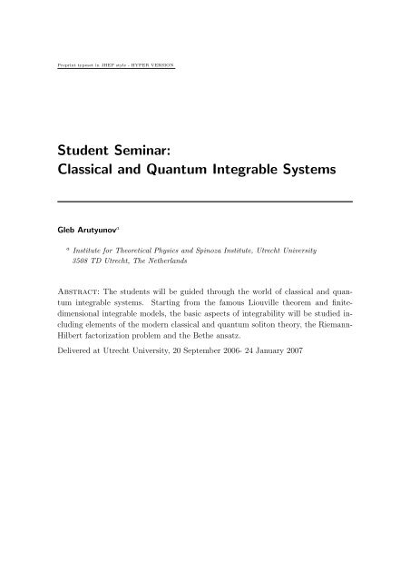
while the Poisson bracket is {p, q} = 1. Energy is conserved, therefore, the phase<br />
space is fibred into ellipses H = E.<br />
p<br />
stationary point<br />
H=E=const −−energy levels<br />
q<br />
HARMONIC OSCILLATOR −− PROTOTYPE OF LIOUVILLE INTEBRABLE SYSTEMS<br />
Problem.<br />
system<br />
Rewrite the Poisson bracket {p, q} = 1 <strong>and</strong> the Hamiltonian in the new coordinate<br />
p = ρ cos(θ) , q = ρ ω sin(θ) .<br />
The answer is<br />
The hamiltonian is<br />
{ρ, θ} = ω ρ .<br />
H = 1 2 ρ2 → ρ = √ 2H .<br />
We see that ρ is an integral of motion. Equation for θ:<br />
˙θ = {H, θ} = ρ{ρ, θ} = ω ⇒ θ(t) = ωt + θ 0 .<br />
This means that the flow takes place on the ellipsis with the fixed value of ρ.<br />
Generalization to n harmonic oscillators is easy:<br />
H =<br />
n∑<br />
i=1<br />
1<br />
2 (p2 i + ω 2 i q 2 i ) .<br />
– 6 –
Commuting integrals<br />
F i = 1 2 (p2 i + ω 2 i q 2 i ) .<br />
Define the common level manifold<br />
M f = {x ∈ M : F i = f i , i = 1, . . . , M}<br />
This manifold is isomorphic to n-dimensional real torus which is a cartesian product<br />
of n topological circles. These tori foliate the phase space <strong>and</strong> can be parametrized<br />
with n angle variables θ i which evolve linearly in time with frequencies ω i . This<br />
motion is conditionally periodic: if all the periods T i = 2π<br />
ω i<br />
are rationally dependent:<br />
T i<br />
T j<br />
= rational number<br />
the motion is periodic, otherwise the flow is dense on the torus.<br />
1.3 The Liouville theorem<br />
The system is Liouville integrable if it possesses n independent conserved quantities<br />
F i , i = 1, . . . , n, {H, F i } which are in involution<br />
{F i , F j } = 0 .<br />
The Liouville theorem. Suppose that we are given n functions in involution on a<br />
symplectic 2n-dimensional manifold<br />
Consider a level set of the functions F i :<br />
F 1 , . . . , F n , {F i , F j } = 0 .<br />
M f = {x ∈ M : F i = f i , i = 1, . . . , n}<br />
Assume that the n functions F i are independent on M f . In other words, the n-forms<br />
dF i are linearly independent at each point of M f . Then<br />
1. M f is a smooth manifold, invariant under the flow with H = H(F i ).<br />
2. If the manifold M is compact <strong>and</strong> connected then it is diffeomorphic to the<br />
n-dimensional torus<br />
T n = {(ψ 1 , . . . , ψ n ) mod 2π}<br />
3. The phase flow with the Hamiltonian function H determines a conditionally<br />
periodic motion on M f , i.e. in angular variables<br />
dψ i<br />
dt = ω i , ω i = ω i (F j ) .<br />
– 7 –
4. The equations of motion with Hamiltonian H can be integrated by quadratures.<br />
Let us outline the proof. Consider the level set of the integrals<br />
M f = {x ∈ M : F i = f i , i = 1, . . . , M} .<br />
By assumptions, the n one-forms dF i are linearly independent at each point of M f ;<br />
by the implicit function theorem, M f is an n-dimensional submanifold on the 2ndimensional<br />
phase space M. Moreover, the n linearly-independent vector fields<br />
ξ Fi = {F i , . . .}<br />
are tangent to M f <strong>and</strong> commute with each other.<br />
Let α = ∑ i p idq i be the canonical 1-form <strong>and</strong> ω = dα = ∑ i dp i ∧ dq i is the<br />
symplectic form on the phase space M. Consider a canonical transformation<br />
i.e.<br />
(p i , q i ) → (F i , ψ i )<br />
ω = ∑ i<br />
dp i ∧ dq i = ∑ i<br />
dF i ∧ dψ i<br />
such that F i are treated as the new momenta. If we found this transformation then<br />
equations of motion read as<br />
˙ F j = {H, F j } = 0 ,<br />
˙ψ j = {H, ψ j } = ∂H<br />
∂F j<br />
= ω j .<br />
Thus, ω i are constant in time. In these coordinates equations of motion are solved<br />
trivially<br />
F j (t) = F j (0) , ψ j (t) = ψ j (0) + tω j .<br />
Thus, we see that the basic problem is to construct a canonical transformation<br />
(p i , q i ) → (F i , ψ i ). This is usually done with the help of the so-called generating<br />
function S. Consider M f : F i (p, q) = f i <strong>and</strong> solve for p i : p i = p i (f, q). Consider the<br />
function<br />
We see that<br />
<strong>and</strong> we further define<br />
S(f, q) =<br />
∫ m<br />
m 0<br />
α =<br />
∫ q<br />
p j = ∂S<br />
∂q j<br />
ψ j = ∂S<br />
∂f j<br />
q 0<br />
∑<br />
i<br />
p i (f, ˜q)d˜q i<br />
– 8 –
Thus, we have<br />
Since d 2 S = 0 we get<br />
i.e. the transformation is canonical.<br />
dS = ∂S<br />
∂q j<br />
dq j + ∂S<br />
∂f j<br />
df j = p j dq j + ψ j df j<br />
∑<br />
dp j ∧ dq j = ∑<br />
j<br />
j<br />
df j ∧ dψ j ,<br />
The next point is to show that S exists, i.e. it does not depend on the path. If<br />
we have a closed path from m 0 to m <strong>and</strong> from m to m 0 <strong>and</strong> assume that M f does<br />
not have non-trivial cycles then by the Stokes theorem we get<br />
∫ m0<br />
∫ ∫<br />
∆S = α = dα = ω = 0<br />
m 0<br />
because the form ω vanishes on M f :<br />
ω(ξ Fi , ξ Fj ) = {F i , F j } = 0 .<br />
In case the manifold M f has non-trivial cycles the situation changes <strong>and</strong> one gets<br />
the change of S given by integral of α over a cycle<br />
∫<br />
∆ cycle S = α<br />
which is a function of F i only! This tells us that in this case the variables ψ j are<br />
multi-valued.<br />
cycle<br />
Mention Darboux<br />
1.4 Action-angle variables<br />
As follows from the Liouville theorem under suitable assumptions of compactness<br />
<strong>and</strong> connectedness motion of a dynamical system in the 2n-dimensional phase space<br />
happens on a n-dimensional torus T n being a common level of n commuting integrals<br />
of motion. The torus has n fundamental cycles C j which allow to introduce the<br />
“normalized” action variables<br />
I j = 1<br />
2π<br />
∮<br />
C j<br />
p i (q, f)dq i ≡ 1<br />
2π<br />
∮<br />
C j<br />
α ,<br />
where f i define the common level T n of the commuting integrals F i . The variables<br />
I j are functions of f i only <strong>and</strong> therefore they are constants of motion. The angle<br />
variables are introduced as independent angle coordinates on the cycles<br />
1<br />
2π<br />
∮<br />
C j<br />
dθ i = δ ij .<br />
– 9 –
Let us show that the variables (I i , θ i ) are canonically conjugate. For that we need<br />
to construct a canonical transformation (p i , q i ) → (I i , θ i ). Consider a generating<br />
function depending on I i <strong>and</strong> q i :<br />
We see that<br />
Let us introduce<br />
S(I, q) =<br />
∫ m<br />
m 0<br />
α =<br />
∫ q<br />
q 0<br />
p i (q ′ , I)dq ′ i .<br />
p j = ∂S<br />
∂q j<br />
=⇒ p = p(q, I).<br />
θ j = ∂S<br />
∂I j<br />
=⇒ θ = θ(q, I).<br />
<strong>and</strong> show that θ j are indeed coincide with the properly normalized angle variables.<br />
We have<br />
∮<br />
1<br />
dθ i = 1 ∮<br />
d ∂S = ∂ ( ∮ 1<br />
)<br />
dS = ∂ ( ∮ 1 ∂S<br />
dq k +<br />
∂S dI k<br />
2π C j<br />
2π C j<br />
∂I i ∂I i 2π C j<br />
∂I i 2π C j<br />
∂q k ∂I<br />
} {{ k<br />
}<br />
Furthermore,<br />
= ∂ ( ∮ 1<br />
)<br />
α = δ ij .<br />
∂I i 2π C j<br />
=0 on C j<br />
)<br />
( ∂S<br />
) (<br />
dI i ∧ dθ i = −d(θ i dI i ) = −d dI i = −d dS − ∂S )<br />
dq i = d(p i dq i ) = dp i ∧ dq i .<br />
∂I i ∂q i<br />
Problem. Find action-angle variables for the harmonic oscillator.<br />
We have<br />
E = 1 2 (p2 + ω 2 q 2 ) =⇒ p(E, q) = ± √ 2E − ω 2 q 2 .<br />
<strong>and</strong>, therefore,<br />
I = 1 ∮<br />
dq √ 2E − ω<br />
2π<br />
2 q 2 = 2<br />
E<br />
2π<br />
∫ √ 2E<br />
ω<br />
− √ 2E<br />
ω<br />
The generating function of the canonical transformation reads<br />
while for the angle variables we obtain<br />
S(I, q) = ω<br />
∫ q<br />
dx √ 2I − x 2 ,<br />
dq √ 2E − ω 2 q 2 = E ω .<br />
θ = ∂S<br />
∂I = ω ∫ q<br />
dx<br />
√<br />
2I − x<br />
2 = ω arctan<br />
q<br />
√<br />
2I − q<br />
2<br />
=⇒ q = √ 2I sin θ ω .<br />
Finally, we explicitly check that the transformation to the action-angle variables is canonical<br />
(<br />
dI<br />
dp ∧ dq = ω √ −<br />
2I − q<br />
2<br />
qdq<br />
)<br />
√ ∧ dq =<br />
2I − q<br />
2<br />
ω<br />
√<br />
2I − q<br />
2 dI ∧ d(√ 2I sin θ ω<br />
)<br />
= dI ∧ dθ .<br />
– 10 –
2. Examples of integrable models solved by Liouville theorem<br />
2.1 Some general remarks<br />
Problem. Consider motion in the potential<br />
V (q) =<br />
Solve eoms <strong>and</strong> find a period of oscillations. One has<br />
t − t 0 =<br />
∫ q<br />
q 0<br />
dq<br />
√<br />
= −<br />
2(E − g2<br />
sin 2 q )<br />
∫ q<br />
q 0<br />
g2<br />
sin 2 q , E > g2 .<br />
d cos q<br />
√ √<br />
2E<br />
(E−g 2 )<br />
E<br />
− cos 2 q<br />
∫ arccos q<br />
= −<br />
arccos q 0<br />
Thus, motion happens on the interval q 0 < q < π − q 0 <strong>and</strong> taking q 0 = arcsin<br />
We see from here that<br />
Period is<br />
cos √ } {{<br />
2E<br />
}<br />
ω<br />
It does not depend on g 2 !!!<br />
t = − 1 √<br />
2E<br />
(<br />
arcsin<br />
x<br />
√<br />
E−g 2<br />
E<br />
( π<br />
t = cos<br />
2 − arcsin x<br />
)<br />
√ =<br />
1 − g2<br />
E<br />
T = 2π ω =<br />
)<br />
2π √<br />
2E<br />
.<br />
| x=cos q<br />
q<br />
E−g<br />
x=<br />
2<br />
E<br />
x<br />
√<br />
1 − g2<br />
E<br />
dx<br />
√ √ .<br />
2E<br />
(E−g 2 )<br />
E<br />
− x 2<br />
√<br />
g 2<br />
E<br />
= √<br />
1<br />
cos q .<br />
1 − g2<br />
E<br />
one gets<br />
Problem. Consider a one-dimensional harmonic oscillator with the frequency ω <strong>and</strong> compute the<br />
area surrounded by the phase curve corresponding to the energy E. Show that the period of motion<br />
along this phase curve is given by T = dS<br />
dE .<br />
A curve is an ellipsis<br />
( x<br />
a<br />
) 2<br />
+<br />
( y<br />
b<br />
) 2<br />
= 1<br />
with the area<br />
S = 2b<br />
∫ a<br />
−a<br />
dx √ ∫ π √<br />
1 − x 2 /a 2 2<br />
= 2ba dφ cos φ 1 − sin 2 φ = 2ab<br />
− π 2<br />
∫ π<br />
2<br />
− π 2<br />
dφ cos 2 φ = πab .<br />
We have to identify a = ρ, b = ρ ω<br />
so that<br />
S = πab = π ρ2<br />
ω = 2π ω E .<br />
From here we see that<br />
dS<br />
dE = 2π ω = T ,<br />
where T is a period of motion. The last expression has the same form as the first law of thermodynamics<br />
dE = 1 T<br />
dS provided that 1/T is the temperature (the period ≡ the inverse temperature).<br />
Problem. Let E 0 be the value of the potential at a minimum point ξ. Find the period T 0 =<br />
lim E→E0 T (E) of small oscillations in a neighborhood of the point ξ.<br />
– 11 –
We have<br />
H = p2<br />
2<br />
p2<br />
+ V (x) =<br />
2 + V } {{ (ξ) + V ′ (ξ)(x − ξ) + 1 } } {{ } 2 V ′′ (ξ)(x − ξ) 2 + · · ·<br />
const =0<br />
Effectively we have motion described by the harmonic oscillator with the Hamiltonian<br />
H eff = p2<br />
2 + 1 2 V ′′ (ξ)q 2<br />
whose frequency is ω = √ V ′′ (ξ). Therefore the period of small oscillations is<br />
T 0 =<br />
2π<br />
√<br />
V<br />
′′<br />
(ξ) .<br />
2.2 The Kepler two-body problem<br />
Here we consider one of the historically first examples of integrable systems solved<br />
by the Liouville theorem: The Kepler two-body problem of planetary motion.<br />
In the center of mass frame eoms are<br />
d 2 x i<br />
dt 2<br />
(r)<br />
= −∂V , r =<br />
∂x i<br />
√<br />
x 2 1 + x 2 2 + x 2 3<br />
In the original Kepler problem V (r) = − k , k > 0. The Hamiltonian<br />
r<br />
H = 1 2<br />
3∑<br />
p 2 i + V (r)<br />
i=1<br />
<strong>and</strong> the bracket {p i , x j } = δ ij .<br />
Problem . Show that the angular momentum<br />
⃗J = (J 1 , J 2 , J 3 ) ,<br />
J ij = x i p j − x j p i = ɛ ijk J k<br />
is conserved.<br />
J˙<br />
ij = ẋ i p j − x i ṗ j − (i ↔ j) = p i p j + ∂V<br />
∂r x ∂r<br />
i − (i ↔ j) = ∂V<br />
∂x j ∂r<br />
Note that this is a consequence of the central symmetry.<br />
(<br />
x i<br />
∂r<br />
∂x j<br />
− x j<br />
∂r<br />
∂x i<br />
)<br />
= 0<br />
Problem. Compute the Poisson brackets<br />
Show that there are three commuting quantities<br />
{J i , J j } = −ɛ ijk J k<br />
H, J 3 , J 2 = J 2 1 + J 2 2 + J 2 3<br />
Rewrite the canonical one form in the polar coordinates<br />
x 1 = r sin θ cos φ, x 2 = r sin θ sin φ, x 3 = r cos θ<br />
– 12 –
We find<br />
α = ∑ i<br />
p i dx i = p r dr + p θ dθ + p φ dφ ,<br />
where the original momenta are expressed as<br />
p 1 = 1 (<br />
sin φ<br />
)<br />
rp r cos φ sin θ + p θ cos θ cos φ − p φ ,<br />
r<br />
sin θ<br />
p 2 = 1 (<br />
cos φ<br />
)<br />
rp r sin φ sin θ + p θ cos θ sin φ + p φ ,<br />
r<br />
sin θ<br />
p 3 = p r cos θ − 1 r p θ sin θ .<br />
Conserved quantities<br />
(<br />
p 2 r + 1 r 2 p2 θ +<br />
H = 1 2<br />
J 2 = p 2 θ + 1<br />
sin 2 θ p2 φ<br />
J 3 = p φ<br />
1<br />
)<br />
r 2 sin 2 θ p2 φ + V (r)<br />
To better underst<strong>and</strong> the physics we note that the motion happens in the plane<br />
orthogonal to the vector J. ⃗ Without loss of generality we can rotate our coordinate<br />
system such that in a new system J ⃗ has only the third component: J ⃗ = (0, 0, J3 ).<br />
This simply accounts in putting in our previous formulae θ = π . Then we note that<br />
2<br />
p 2 φ<br />
˙φ = {H, φ} = {<br />
2r 2 sin 2 θ , φ} =<br />
that for θ = π 2 expresses the integral of motion p φ as<br />
p φ = r 2 ˙φ.<br />
p φ<br />
r 2 sin 2 θ<br />
This is the conservation law of angular momentum discovered by Kepler through<br />
observations of the motion of Mars. The quantity p φ = J has a simple geometric<br />
meaning. Kepler introduced the sectorial velocity C:<br />
C = dS<br />
dt ,<br />
where ∆S is an area of the infinitezimal sector swept by the radius-vector ⃗r for time<br />
∆t:<br />
∆S = 1 2 r · r ˙φ∆t + O(∆t 2 ) ≈ 1 2 r2 ˙φ∆t .<br />
This is the (second) law discovered by Kepler: in equal times the radius vector sweeps<br />
out equal areas, so the sectorial velocity is constant. This is one of the formulations<br />
of the conservation law of angular momentum. 1<br />
1 Some satellites have very elongated orbits. According to Kepler’s law such a satellite spends<br />
most of its time in the distant part of the orbit where the velocity ˙φ is small.<br />
– 13 –
We can now see how the solution can be found by using the general approach<br />
based on the Liouville theorem. The expressions for the momenta on the surface of<br />
constant energy <strong>and</strong> J = J 3 are<br />
√<br />
p r = 2(H − V ) − J 2<br />
r , p 2 φ = J 3 = J .<br />
We can thus construct the generating function of the canonical transformation from<br />
from the Liouville theorem<br />
∫ r<br />
S =<br />
√2(H − V ) − J ∫ 2 φ<br />
r + Jdφ<br />
2<br />
<strong>and</strong> the associated angle variables<br />
We have eoms<br />
Integrating the first one we obtain<br />
ψ H = ∂S<br />
∂H ,<br />
ψ J = ∂S<br />
∂J<br />
˙ψ H = 1 , ˙ψ J = 0 .<br />
<strong>and</strong>, therefore,<br />
The equation for ψ J gives<br />
ψ J = −<br />
t − t 0 =<br />
∫ r<br />
ψ H = t − t 0<br />
∫ r<br />
dr<br />
√<br />
.<br />
2(H − V ) − J2<br />
r 2<br />
Jdr<br />
√<br />
+ φ = 0 ,<br />
r 2 2(H − V ) − J2<br />
r 2<br />
so that<br />
φ =<br />
∫ r<br />
Jdr<br />
√<br />
r 2 2 ( ) .<br />
E − V (r) − J 2<br />
2r 2<br />
Generically, equation which defines the values of r at which ṙ = 0:<br />
E − V (r) − J 2<br />
2r 2 = 0<br />
has two solutions: r min <strong>and</strong> r max , they are called pericentum <strong>and</strong> apocentrum respectively<br />
2 . When ṙ = 0, ˙φ ≠ 0. The r oscillates monotonically between rmin <strong>and</strong><br />
2 If the earth is the center then r min <strong>and</strong> r max are called perigee <strong>and</strong> apogee, if the sun – perihelion<br />
<strong>and</strong> apohelion, if the moon – perilune <strong>and</strong> apolune.<br />
– 14 –
max while φ changes monotonically. The angle between neighboring apocenter <strong>and</strong><br />
pericenter is given by<br />
∆φ =<br />
∫ rmax<br />
r min<br />
Jdr<br />
√<br />
r 2 2 ( ) .<br />
E − V (r) − J2<br />
2r 2<br />
Generic orbit is not closed! It is closed only if ∆φ = 2π m , m, n ∈ Z, otherwise it is<br />
n<br />
everywhere dense in the annulus. The annulus might degenerate into a circle.<br />
2.2.1 Central fields in which all bounded orbits are closed.<br />
Determination of a central potential for which all bounded orbits are closed is called<br />
the I.L.F. Bertr<strong>and</strong> problem.<br />
There are only two cases for which bounded orbits are closed<br />
V (r) = ar 2 , a ≥ 0 ,<br />
V (r) = − k r , k ≥ 0 .<br />
To show this we have to solve several problems.<br />
Problem. Show that the angle φ between the pericenter <strong>and</strong> apocenter is equal to the half-period<br />
of an oscillation in the one dimensional system with potential energy W (x) = V (J/x) + x2<br />
2 .<br />
Substitution r = J r gives ∆φ =<br />
∫ xmax<br />
x min<br />
dx<br />
√<br />
2(E − W (x))<br />
.<br />
Problem. Find the angle φ for an orbit close to the circle of radius r.<br />
Effectively the angle φ is described by half-period of oscillation<br />
∆φ =<br />
∫ xmax<br />
x min<br />
dx<br />
√<br />
2(E − W (x))<br />
.<br />
We have<br />
∆φ = π ω , ω = √ W ′′ (x) ,<br />
where x = J r . We find W ′ (x) = ∂ x V (J/x) + x = − J x 2 V ′ (J/x) + x ,<br />
We have to take<br />
W ′′ (x) = 2 J x 3 V ′ (J/x) + J 2<br />
x 4 V ′′ (J/x) + 1 .<br />
− J x 2 V ′ (J/x) + x = 0 =⇒ x3<br />
J = V ′ (J/x) =⇒ J<br />
r 3/2 = √ V ′ (r) .<br />
– 15 –
Thus,<br />
<strong>and</strong>, therefore, the half-period is<br />
W ′′ (x) = J )<br />
(3V ′<br />
x 3 (r) + rV ′′ (r) = 3V ′ (r) + rV ′′ (r)<br />
V ′ (r)<br />
√<br />
V<br />
∆φ circ = π<br />
′ (r)<br />
3V ′ (r) + rV ′′ (r) .<br />
Problem. Find the potentials V for which the magnitude of ∆φ circ does not depend on the radius.<br />
We have to require<br />
( 3V ′ (r) + rV ′′ (r)<br />
V ′ (r)<br />
) ′ ( rV ′′ (r)<br />
) ′ (<br />
= =<br />
V ′ r ( log V ′ (r) ) ) ′<br />
′<br />
= 0 ,<br />
(r)<br />
i.e.<br />
log V ′ (r) = const<br />
∫ 1<br />
r<br />
= s log r + m , s, m = const .<br />
Further,<br />
V ′ (r) = const r s , =⇒ V (r) = ar α ,<br />
or V (r) = b log r if s = −1. Finally, the expression<br />
V (r) = ar α we will get<br />
V ′ (r)<br />
3V ′ (r)+rV ′′ (r)<br />
should be positive. If we take<br />
V ′ (r)<br />
3V ′ (r) + rV ′′ (r) = α<br />
3α + α(α − 1) = 1 > 0 =⇒ α > −2 .<br />
2 + α<br />
Finally, we also have<br />
∆φ circ =<br />
π<br />
√ 2 + α<br />
.<br />
Here the logarithmic case correspond to α = 0. Particular cases are α = 2 which gives ∆φ circ = π 2<br />
<strong>and</strong> α = −1 which gives ∆φ circ = π.<br />
Problem. Let V (r) → ∞ as r → ∞. Find<br />
lim ∆φ circ(E, J)<br />
E→∞<br />
Let us make a substitution x = yx max , we get<br />
∫ 1<br />
dy<br />
∆φ circ = √<br />
y min 2(Q(1) − Q(y))<br />
(<br />
where Q(y) = y2<br />
2 + 1 J<br />
x<br />
V 2<br />
max yx max<br />
). As E → ∞ we have x max → ∞ <strong>and</strong> y min → 0 <strong>and</strong> the second<br />
term in Q can be discarded. Thus, we get<br />
∆φ circ =<br />
∫ 1<br />
0<br />
dy<br />
√<br />
1 − y<br />
2 = π 2 .<br />
Problem. Let V (r) = −kr −β , where 0 < β < 2. Find<br />
lim ∆φ circ(E, J)<br />
E→−0<br />
– 16 –
One has<br />
∆φ circ =<br />
∫ xmax<br />
x min<br />
dx<br />
√<br />
2E + 2k x<br />
J β − x 2<br />
β<br />
E→0<br />
→<br />
∫ xmax<br />
x min<br />
dx<br />
√<br />
2k<br />
x<br />
J β − x 2<br />
β<br />
Rescale x = αy with α satisfying the relation 2k<br />
J β α β = α 2 , then we get<br />
∆φ circ =<br />
∫ 1<br />
We note that the result does not depend on J.<br />
0<br />
dy<br />
√<br />
yβ − y = π<br />
2 2 − β .<br />
Now we are ready to find the potentials for which all bounded orbits are closed. If<br />
all bounded orbits are closed, then, in particular, ∆φ circ = 2π m = const. That means<br />
n<br />
that ∆φ circ should not depend on the radius, which is the case for the potentials<br />
V (r) = ar α , α > −2 <strong>and</strong> V (r) = b log r .<br />
In both cases ∆φ circ = √ π<br />
2+α<br />
. If α > 0 then lim E→∞ ∆φ circ (E, J) = π <strong>and</strong> therefore<br />
2<br />
α = 2. If α < 0 then lim E→0 ∆φ circ (E, J) = π . Then we have an equality<br />
2+α<br />
π<br />
= √ π<br />
2+α 2+α<br />
which gives α = −1. In the case α = 0 we find ∆φ circ = √ π 2<br />
which<br />
is not commensurable with 2π. Therefore all bounded orbits are closed only for<br />
V = ar 2 <strong>and</strong> U = − k .<br />
r 2<br />
2.2.2 The Kepler laws<br />
For the original Kepler problem we have<br />
<strong>and</strong><br />
Integrating we get<br />
∫<br />
φ =<br />
V (r) = − k r + J 2<br />
2r 2 .<br />
Jdr<br />
√<br />
r 2 2(E + k − J 2<br />
)<br />
r 2r 2<br />
φ = arccos<br />
J<br />
√ − k r J<br />
.<br />
2E + k2<br />
J 2<br />
An integration constant is chosen to be zero which corresponds to the choice of an<br />
origin of reference for the angle φ at the pericenter. Introduce the notation<br />
√<br />
J 2<br />
k = p , 1 + 2EJ 2<br />
= e ,<br />
k 2<br />
This leads to<br />
r =<br />
p<br />
1 + e cos φ<br />
– 17 –
This is the so-called focal equation of a conic section. When e < 1, i.e. E < 0, the<br />
conic section is an ellipse. The number p is called a parameter of the ellipse <strong>and</strong> e<br />
the essentricity. The motion is bounded for E < 0.<br />
The semi-axis a is determined as<br />
2a =<br />
p<br />
1 − e + p<br />
1 + e = 2p<br />
1 − e . 2<br />
We also have<br />
Thus,<br />
c = a −<br />
p<br />
1 + e = 1 ( p<br />
2 1 − e − p )<br />
= ep<br />
1 + e 1 − e . 2<br />
c<br />
a = e .<br />
b a p<br />
c O<br />
p<br />
p<br />
1−e 1+e<br />
Keplerian ellipse<br />
Obviously, we have three distinguished points<br />
φ = 0 : r = p<br />
1 + e ,<br />
φ = π 2 : r = p ,<br />
We can now formulate the Kepler laws:<br />
φ = π : r = p<br />
1 − e .<br />
1. The first law: Planets describe ellipses with the Sun at one focus.<br />
2. The second law: The sectorial velocity is constant.<br />
3. The third law: The period of revolution around an elliptical orbit depends only<br />
on the size of the major semi-axes. The squares of the revolution periods of<br />
two planets on different elliptical orbits have the same ratio as the cubes of<br />
their major semi-axes.<br />
Let us prove the third law. Let T be a revolutionary period <strong>and</strong> S be the area swept<br />
out by the radius vector over the period. We have<br />
S = πab = πa 2√ √<br />
1 − e 2 = π 1 − e2 = π<br />
(1 − e 2 ) 2 (1 − e 2 ) 3 2<br />
p 2<br />
p 2<br />
= πkJ<br />
( √ 2|E|) 3 ,<br />
– 18 –
while<br />
i.e.<br />
a =<br />
p<br />
1 − e = k<br />
2 2|E| .<br />
On the other h<strong>and</strong>, since the sectorial velocity C is constant we have<br />
∫ T<br />
0<br />
C =<br />
∫ T<br />
0<br />
dt dS<br />
dt = S , =⇒ CT = J 2 T = S ,<br />
T = 2S J =<br />
2πk<br />
( √ 2|E|) = √ 2π a 3 2 .<br />
3 k<br />
It is interesting to note that the total energy depends only on the major semi-axis<br />
a <strong>and</strong> it is the same for the whole set of elliptical orbits from a circle of radius a<br />
to a line segment of length 2a. The value of the second semi-axis do depend on the<br />
angular momentum.<br />
The Runge-Lenz vector <strong>and</strong> the Liouville torus. The phase space of the motion in the<br />
central field is T ∗ R 3 , i.e. it is six-dimensional. There are four conserved integrals:<br />
three components of the angular momentum J i <strong>and</strong> the energy E. This shows that<br />
the motion happens on the two-dimensional manifold. In case of the bounded motion<br />
it is the two-dimensional Liouville torus. Thus, there are two frequencies associated<br />
<strong>and</strong> when they are not rationally commensurable the orbits are not closed but rather<br />
dense on the torus. For the specific Kepler motion (with any sign of k) there is one<br />
more non-trivial conserved quantity appears which is absent for a generic central<br />
potential: The Runge-Lenz vector (for definiteness we assume that k > 0):<br />
⃗R = ⃗v × ⃗ J − k ⃗r r .<br />
Problem. Show that the Runge-Lenz vector is conserved.<br />
Indeed, we have<br />
˙⃗R = ˙⃗v ×<br />
}{{}<br />
J ⃗ −k ⃗v r + k⃗r(⃗v⃗r) r 3<br />
m ⃗r×⃗v<br />
= m ˙⃗v × (⃗r × ⃗v) − k ⃗v r + k⃗r(⃗v⃗r) r 3 .<br />
On the other h<strong>and</strong>,<br />
m ˙⃗v = − ∂U ⃗r<br />
∂r r = −k ⃗r r 3<br />
<strong>and</strong>, therefore,<br />
˙⃗R = −k 1 r 3 ⃗r × (⃗r × ⃗v) − k⃗v r + k⃗r(⃗v⃗r) r 3<br />
Further one has to use the formula<br />
⃗r × (⃗r × ⃗v) = (⃗v⃗r)⃗r − r 2 ⃗v<br />
– 19 –
to show that ˙⃗ R = 0. The last formula can be proved by noting that the vector<br />
⃗r × (⃗r × ⃗v) = α⃗r + β⃗v<br />
is orthogonal to ⃗r. Thus, multiplying both sides by ⃗r we get<br />
0 = αr 2 + β(⃗v⃗r) .<br />
On the other h<strong>and</strong>, multiplying both sides by ⃗v we get<br />
(⃗v, ⃗r × (⃗r × ⃗v)) = α(⃗v⃗r) + βv 2<br />
which gives<br />
(⃗v, ⃗r × (⃗r × ⃗v)) = −(⃗r × ⃗v, ⃗r × ⃗v = −r 2 v 2 sin φ = −r 2 v 2 (1 − cos 2 φ)<br />
= −r 2 v 2 + (⃗v⃗r) 2 = α(⃗v⃗r) + βv 2 .<br />
These two equations allows one to find<br />
α = (⃗v⃗r) , β = −r 2 .<br />
2.3 Rigid body<br />
2.3.1 Moving coordinate system<br />
Let K <strong>and</strong> k will be two oriented Euclidean spaces. A motion of K relative to k is<br />
a mapping smoothly depending on t:<br />
D t : K → k ,<br />
which preserves the metric <strong>and</strong> orientation. Every motion can be uniquely written<br />
as the composition of a rotation (D t which maps the origin of K into the origin<br />
of k, i.e. D t is linear mapping) <strong>and</strong> a translation C t : k → k. Let call K <strong>and</strong> k<br />
moving <strong>and</strong> stationary coordinate systems respectively. Let q(t) <strong>and</strong> Q(t) will be the<br />
radius-vector of a point in a stationary <strong>and</strong> moving coordinate systems respectively.<br />
Then<br />
q(t) = D t Q(t) = B t Q(t) + r(t) .<br />
} {{ } }{{}<br />
rotation translation<br />
Differentiating we get an addition formula for velocities<br />
˙q =<br />
ḂQ +B<br />
}{{}<br />
˙Q + ṙ .<br />
transferred rotation<br />
Suppose a point does not move w.r.t. to the moving frame, i.e.<br />
r = ṙ = 0. Then<br />
˙q = ḂQ = ḂB−1 q = Aq ,<br />
˙Q = 0 <strong>and</strong> also that<br />
– 20 –
where A : k → k is a linear operator on k. Since B is a rotation, it is an orthogonal<br />
transformation: BB t = 1. Differentiating w.r.t to t we get<br />
ḂB t + BḂt = 0 =⇒ ḂB −1 + (ḂB−1 ) t = 0 ,<br />
i.e. A is skew-symmetric. On the other h<strong>and</strong>, every skew-symmetric operator from<br />
R 3 to R 3 is the operator of vector multiplication by a fixed vector ω:<br />
˙q = ω × q .<br />
Generically ω depends on t. Thus, in the case of purely rotational motion with ˙Q ≠ 0<br />
we will have<br />
˙q = ω × q + B ˙Q = ω × q<br />
} {{ }<br />
transferred velocity<br />
+ }{{} v ′<br />
relative velocity<br />
.<br />
2.3.2 Rigid bodies<br />
A rigid body is a system of point masses, constrained by holonomic relations expressed<br />
by the fact that the distance between points is constant<br />
|x i − x j | = r ij = const .<br />
If a rigid body moves freely then its center of mass moves uniformly <strong>and</strong> linearly.<br />
A rigid body rotates about its center of mass as if the center of mass were fixed at<br />
a stationary point O. In this way the problem is reduced to a problem with three<br />
degrees of freedom – motion of a rigid body around a fixed point O. The problem of<br />
rotation of rigid body can be studied in more generality without assuming that the<br />
fixed point coincides with the center of mass of a body. Since the Lagrangian function<br />
is invariant under all rotations around O by Noether theorem the components of the<br />
angular momentum M are conserved: Ṁ = 0 . The total energy which is equal to<br />
the kinetic energy is also conserved. Thus, we see that<br />
In the problem of motion of rigid body around a fixed point, in the absence of<br />
outside forces, there are four integrals of motion: three components on M <strong>and</strong> the<br />
energy. Thus, motion happens on a two-dimensional space inside the six-dimensional<br />
phase-space (three rotation angles plus three velocities) :<br />
M f = {M x = f 1 , M y = f 2 , M z = f 3 , E = f 4 > 0 }.<br />
The phase space is a cotangent bundle to SO(3). The manifold M f is invariant: if<br />
the initial conditions of motion give a point on M f then for all time of motion the<br />
point in T SO(3) corresponding to the position <strong>and</strong> velocity of the body remains in<br />
M f . The two-dimensional manifold M f admits a globally defined vector field (this<br />
is the field of velocities of the motion on T SO(3)), it is orientable <strong>and</strong> compact (E<br />
– 21 –
is the bounded kinetic energy). According to the known theorem in topology, a<br />
two-dimensional compact orientable manifold admitting globally defined vector field<br />
is isomorphic to a torus. This is our Liouville torus 3 . According to the Liouville<br />
theorem motion on the torus will be characterized by two frequencies ω 1 <strong>and</strong> ω 2 . If<br />
their ratio is not a rational number then the body never returns to its original state<br />
of motion.<br />
Consider a rigid body rotation around a fixed point O <strong>and</strong> denote by K a coordinate<br />
system rotating with the body around O: in K the body is at rest. Every<br />
vector in K is carried to k by an operator B. By definition of the angular momentum<br />
we have<br />
M = q × m ˙q = m q × (ω × q) .<br />
Denote by J <strong>and</strong> by Ω the angular momentum <strong>and</strong> angular velocity in the moving<br />
frame K. We have<br />
J = m Q × (Ω × Q) .<br />
This defines a linear map A: K → K such that AΩ = J. This operator is symmetric:<br />
(AX, Y ) = (m Q × (X × Q), Y ) = m(Q × X, Q × Y )<br />
because the r.h.s. is symmetric function of X, Y . The operator A is called the inertia<br />
tensor. We see that taking X = Y = Ω we get<br />
E = T = 1 2 (AΩ, Ω) = 1 2 (J, Ω) = m 2 (Q × Ω, Q × Ω) = m 2 ˙Q 2 = m 2 ˙q2 .<br />
being a symmetric operator A is diagonalizable <strong>and</strong> it defines three mutually orthogonal<br />
characteristic directions. In the basis where A is diagonal the inertia operator<br />
<strong>and</strong> the kinetic energy take a very simple form<br />
J i = I i Ω i ,<br />
T = 1 3∑<br />
I i Ω 2 i .<br />
2<br />
The axes of this particular coordinate system are called the principle inertia axes.<br />
Problem. Rewrite expression for energy via the quantities of the stationary frame k.<br />
We have<br />
i=1<br />
E = 1 2 (AΩ, Ω) = 1 2 (J, Ω) = 1 2 (M, ω) = m 2 (q × (q × ω), ω) = m (q × ω, q × ω)<br />
2<br />
= 1 (ω<br />
2 m 2 q 2 − (ωq) 2) = 1 )<br />
2 ω iω j m<br />
(x 2 i δ ij − x i x j .<br />
} {{ }<br />
inertia tensor<br />
3 We cannot use the Liouville theorem to derive this result, because the integrals M i do not<br />
commute with each other <strong>and</strong>, therefore, the Frobenious theorem cannot be applied to deduce that<br />
the level set is a smooth manifold. Nevertheless we can identify the Liouville torus by different<br />
means.<br />
– 22 –
2.3.3 Euler’s top<br />
Consider the motion of a rigid body around a fixed point O. Let J <strong>and</strong> Ω will be<br />
the vector of angular momentum <strong>and</strong> the angular momentum in the body, i.e. in the<br />
moving coordinate system K. We have AΩ = J, where A is the inertia tensor. The<br />
angular momentum M = B t J of the body in space is preserved. Thus, we have<br />
0 = Ṁ = ḂJ + B ˙ J = ḂB−1 M + B ˙ J = ω × M + B ˙ J = B<br />
(<br />
Ω × J + J ˙<br />
)<br />
.<br />
From here we find<br />
dJ<br />
dt = J × Ω = J × A−1 J .<br />
These are the famous Euler equations which describe the motion of the angular momentum<br />
insider the rigid body. If one takes the coordinate adjusted to the principle<br />
axes then one gets the following system of equations<br />
dJ 1<br />
= a 1 J 2 J 3 ,<br />
dt<br />
dJ 2<br />
= a 2 J 3 J 1 ,<br />
dt<br />
dJ 3<br />
= a 3 J 1 J 2 .<br />
dt<br />
Here<br />
a 1 = I 2 − I 3<br />
, a 2 = I 3 − I 1<br />
, a 3 = I 1 − I 2<br />
.<br />
I 2 I 3 I 1 I 3 I 1 I 2<br />
In this way the Euler equations can be viewed as equations for the components of<br />
the angular momentum insider the body.<br />
Consider the energy<br />
H = 1 2 (J, A−1 J) = 1 2<br />
3∑<br />
i=1<br />
J 2 i<br />
I i<br />
.<br />
It is easy to verify explicitly that it is conserved due to eoms:<br />
3∑ J<br />
(<br />
i a1<br />
Ḣ = J i = J 1 J 2 J 3 + a 2<br />
+ a )<br />
3<br />
= 0 .<br />
I i I 1 I 2 I 3<br />
i=1<br />
Verify the conservation of the length of the angular momentum<br />
3∑<br />
(<br />
)<br />
J˙<br />
2 = J i J˙<br />
i = J 1 J 2 J 3 a 1 + a 2 + a 3 = 0 .<br />
i=1<br />
This is of course agrees with the fact that M is conserved <strong>and</strong> that M 2 = J 2 . Thus,<br />
we have proved that the Euler equations have two quadratic integrals: the energy<br />
<strong>and</strong> M 2 = J 2 . Thus, J lies on the intersection of an ellipsoid <strong>and</strong> a sphere:<br />
2E = J 2 1<br />
I 1<br />
+ J 2 2<br />
I 2<br />
+ J 2 3<br />
I 3<br />
, J 2 = J 2 1 + J 2 2 + J 2 3 .<br />
– 23 –
One can study the structure of the curves of intersection by fixing the ellipsoid E > 0<br />
<strong>and</strong> changing the radius J of the sphere.<br />
Note that alternatively the Euler equations can be rewritten as the equations for<br />
the angular velocity Ω:<br />
dΩ 1<br />
dt + I 3 − I 2<br />
Ω 2 Ω 3 = 0 ,<br />
I 1<br />
dΩ 2<br />
dt + I 1 − I 3<br />
Ω 3 Ω 1 = 0 ,<br />
I 2<br />
dΩ 3<br />
dt + I 2 − I 1<br />
Ω 1 Ω 2 = 0.<br />
I 3<br />
We could express Ω 1 <strong>and</strong> Ω 3 from the conservation laws<br />
Ω 2 1<br />
(<br />
)<br />
1 =<br />
(2EI 3 − J 2 ) − I 2 (I 3 − I 2 )Ω 2 2 ,<br />
I 1 (I 3 − I 1 )<br />
Ω 2 1<br />
(<br />
)<br />
3 =<br />
(J 2 − 2EI 1 ) − I 2 (I 2 − I 1 )Ω 2 2 .<br />
I 3 (I 3 − I 1 )<br />
Then plugging this into the Euler equation for Ω 2 we obtain<br />
dΩ 2<br />
dt<br />
=<br />
√<br />
1 ( )(<br />
)<br />
√ (2EI 3 − J 2 ) − I 2 (I 3 − I 2 )Ω 2 2 (J 2 − 2EI 1 ) − I 2 (I 2 − I 1 )Ω 2 2 .<br />
I 2 I1 I 3<br />
We assume that I 3 > I 2 > I 1 <strong>and</strong> further that M 2 > 2EI 2 . Then making the<br />
substitutions<br />
√<br />
√<br />
(I 3 − I 2 )(J<br />
τ = t<br />
− 2EI 1 )<br />
I 2 (I 3 − I 2 )<br />
, s = Ω 2<br />
I 1 I 2 I 3 2EI 3 − J 2<br />
<strong>and</strong> introducing the positive parameter k 2 < 1 by<br />
we obtain<br />
k 2 = (I 2 − I 1 )(2EI 3 − J 2 )<br />
(I 3 − I 2 )(J 2 − 2EI 1 )<br />
τ =<br />
∫ s<br />
0<br />
ds<br />
√<br />
(1 − s2 )(1 − k 2 s 2 ) .<br />
The initial time τ = 0 is chosen such that for s = 0 one has Ω 2 = 0. Inverting the<br />
last integral one gets the Jacobi elliptic function 4<br />
Using two other elliptic functions<br />
s = sn τ .<br />
cn 2 τ + sn 2 τ = 1 , dn 2 τ + k 2 sn 2 τ = 1<br />
4 Elliptic functions were first applied to this problem in Rueb, Specimen inaugural, Utrecht, 1834.<br />
– 24 –
we obtain the solution<br />
Ω 1 =<br />
Ω 2 =<br />
Ω 3 =<br />
√<br />
2EI 3 − J 2<br />
I 1 (I 3 − I 1 ) cn τ ,<br />
√<br />
2EI 3 − J 2<br />
I 2 (I 3 − I 1 ) sn τ ,<br />
√<br />
J 2 − 2EI 1<br />
I 3 (I 3 − I 1 ) dn τ .<br />
Period of all these three elliptic functions is given by 4K, where K is the complete<br />
elliptic integral of the first kind:<br />
K =<br />
∫ 1<br />
0<br />
ds<br />
√<br />
(1 − s2 )(1 − k 2 s 2 ) .<br />
Period in time t is therefore given by<br />
√<br />
I 1 I 2 I 3<br />
T = 4K<br />
(I 3 − I 2 )(J 2 − 2EI 1 ) .<br />
After this time both Ω <strong>and</strong> J will return to their original values. Thus, Ω or J<br />
perform a strictly periodic motion. What is remarkable, is that the top itself does<br />
not return in its original position in the stationary coordinate system k.<br />
We have obtained that the angular momentum J moves periodically with the<br />
period T . On the other h<strong>and</strong>, we know that the Liouville torus has the dimension<br />
two! This means that the actual motion of the body should be parameterized by two<br />
frequencies ω 1,2 . Let us express the angular velocity Ω via the Euler angles <strong>and</strong> their<br />
derivatives. Let x 1 , x 2 , x 3 be the axes of the moving frame k. Components of ˙θ on<br />
x 1 are<br />
˙θ 1 = ˙θ cos ψ , ˙θ2 = − ˙θ sin ψ , ˙θ3 = 0 .<br />
The velocity ˙φ is directed along Z. Its projections are<br />
˙φ 1 = ˙φ sin θ sin ψ , ˙φ2 = ˙φ sin θ cos ψ , ˙φ3 = ˙φ cos θ .<br />
Finally, the velocity ˙ψ is directed along x 3 . Thus, we can write the components of<br />
the angular velocity in the moving frame as<br />
Ω 1 = ˙φ sin θ sin ψ + ˙θ cos ψ<br />
Ω 2 = ˙φ sin θ cos ψ − ˙θ sin ψ<br />
Ω 3 = ˙φ cos θ + ˙ψ .<br />
– 25 –
Substituting these formula into the expression for the kinetic energy T = 1I 2 iΩ 2 i<br />
obtain the kinetic energy in terms of the Euler angles.<br />
we<br />
Problem. By using Euler angles relate the angular momenta in the moving <strong>and</strong> the stationary<br />
coordinate systems. The momentum M is directed along the Z axis of the stationary coordinate<br />
system.<br />
We have<br />
M sin θ sin ψ = I 1 Ω 1 ,<br />
M sin θ cos ψ = I 2 Ω 2 ,<br />
M cos θ = I 3 Ω 3 .<br />
From here<br />
cos θ = I 3Ω 3<br />
M , tan ψ = I 1Ω 1<br />
I 2 Ω 2<br />
.<br />
Solution of the last problem allows one to find<br />
√<br />
I 3 (M<br />
cos θ =<br />
2 − 2EI 1 )<br />
dn τ ,<br />
M 2 (I 3 − I 1 )<br />
√<br />
I 1 (I 3 − I 2 ) cn τ<br />
tan ψ =<br />
I 2 (I 3 − I 1 ) sn τ .<br />
Thus, both angles θ <strong>and</strong> ψ are periodic functions of time with the period T (the same<br />
period as for Ω!). However, the angle φ does not appear in the formulas relating the<br />
angular momenta in the moving <strong>and</strong> the stationary coordinate systems. We can find<br />
it from<br />
Ω 1 = ˙φ sin θ sin ψ + ˙θ cos ψ<br />
Ω 2 = ˙φ sin θ cos ψ − ˙θ sin ψ .<br />
Solving we get<br />
˙φ = Ω 1 sin ψ + Ω 2 cos ψ<br />
.<br />
sin θ<br />
This leads to the differential equation<br />
dφ<br />
dt = M I 1Ω 2 2 + I 2 Ω 2 2<br />
.<br />
I1Ω 2 2 1 + I2Ω 2 2 2<br />
Thus, solution is given by quadrature but the integr<strong>and</strong> contains elliptic functions in<br />
a complicated way. One can show that the period of φ, which is T ′ is not comparable<br />
with T . This leads to the fact that the top never returns to its original state. The<br />
periods T <strong>and</strong> T ′ are the periods of motion over the Liouville torus.<br />
– 26 –
2.3.4 On the Jacobi elliptic functions<br />
Consider a trigonometric integral<br />
y = sin −1 x =<br />
∫ x<br />
0<br />
∫<br />
dy<br />
arcsin φ<br />
√ = d sin φ<br />
√<br />
1 − y<br />
2 1 − sin 2 φ .<br />
If −1 ≤ Rex ≤ 1 this integral coincides with the function y = arcsin x.<br />
0<br />
Upper−half plane<br />
.><br />
><br />
−1<br />
><br />
0<br />
sin −1<br />
><br />
+1<br />
><br />
Image of the<br />
upper−half plane<br />
−<br />
+<br />
−<br />
− Pi/2<br />
> ><br />
0<br />
Pi/2<br />
+<br />
−<br />
+<br />
This integral maps the punctured (at ±1)upper-half plane one-to-one onto the shaded<br />
strip. The integral is inverted by the function sin which is period with the period<br />
∫ 1<br />
dy<br />
2π = 4 × complete integral √ .<br />
0 1 − y<br />
2<br />
Thus, sin can be viewed as the function on the complex cylinder X = C/L with<br />
L = 2πZ . It also gives a Riemann map of the strip |x| < π , y > 0 to the upper-half<br />
2<br />
plane, st<strong>and</strong>ardized by the values 0, 1, ∞ at 0, π, i∞. 2<br />
It is remarkable discovery of Gauss <strong>and</strong> Abel that the same picture holds for the<br />
incomplete integral of the first kind:<br />
x →<br />
∫ x<br />
0<br />
dy<br />
√<br />
(1 − y2 )(1 − k 2 y 2 ) .<br />
The case k = 0 is trigonometric we have discussed above. The novel point is that<br />
for k 2 ≠ 0, 1 the inversion of the integral now leads to an elliptic function, that is a<br />
single-valued function having not just one but two independent complex periods.<br />
– 27 –
Upper−half plane<br />
01 01 0 0 1 1 01<br />
−1/k<br />
−1<br />
1<br />
1/k<br />
sn x<br />
K−i K’<br />
K+i K’<br />
+<br />
−K<br />
K<br />
The rectangle region is mapped by the Jacobi function sn x one-to-one onto the<br />
upper-half-plane with four punctures.<br />
The mapping of the upper half-plane onto the rectangle is such that the points<br />
0, 1, 1/k, ∞, −1/k, −1 have the images 0, K, K + iK ′ , iK ′ , K − iK ′ , −K respectively.<br />
The function sn x repeats in congruent blocks of four rectangles <strong>and</strong>, therefore, is<br />
invariant under translations by ω 1 = 4K(k) <strong>and</strong> ω 3 = 2iK ′ (k). Here K <strong>and</strong> K ′ are<br />
complete elliptic integrals (K ′ is called complementary)<br />
K =<br />
K ′ =<br />
∫ 1<br />
0<br />
∫ 1/k<br />
1<br />
dy<br />
√<br />
(1 − y2 )(1 − k 2 y 2 )<br />
∫<br />
dy<br />
1<br />
√<br />
(1 − y2 )(1 − k 2 y 2 ) =<br />
where k = √ 1 − k 2 is the complementary modulus.<br />
Writing<br />
x =<br />
∫ sn x<br />
<strong>and</strong> differentiating over x we will get<br />
0<br />
1 =<br />
dy<br />
√<br />
(1 − y2 )(1 − k 2 y 2 )<br />
sn ′ x<br />
√<br />
(1 − y2 )(1 − k 2 y 2 )<br />
0<br />
dy<br />
√<br />
(1 − y2 )(1 − k ′2 y 2 ) ,<br />
or<br />
(sn ′ x) 2 = (1 − y 2 )(1 − k 2 y 2 ) .<br />
This is differential equation satisfied by the Jacobi elliptic function sn x.<br />
– 28 –
2.3.5 Mathematical pendulum<br />
The theory of elliptic functions finds beautiful applications in many classical problems.<br />
One of them is the motion of the mathematical pendulum in the gravitational<br />
field of the Earth.<br />
Consider the mathematical pendulum (of mass M) in the gravitational field of<br />
the Earth.<br />
L<br />
01<br />
01<br />
M<br />
A pendulum in the gravitational field of the Earth. Here L is its length <strong>and</strong> G is<br />
the gravitational constant.<br />
G<br />
First we derive the eoms. The radius-vector <strong>and</strong> the velocity are is<br />
⃗r(t) = (L} sin {{ θ}<br />
, L} cos {{ θ}<br />
) , ⃗v(t) = (L cos θ ˙θ, −L sin θ ˙θ) .<br />
x y<br />
Projecting the Newton equations of the axes x <strong>and</strong> y we find<br />
Differentiating we get<br />
L d2 cos θ<br />
dt 2 = mg , L d2 sin θ<br />
dt 2 = 0 .<br />
−L(cos θ ˙θ 2 + sin θ¨θ) = mg , − sin θ ˙θ 2 + cos θ¨θ = 0 .<br />
Excluding from these equations ˙θ 2 we obtain the equations of motion<br />
L¨θ = −mg sin θ .<br />
This equation can be integrated once by noting that<br />
i.e. that<br />
d ˙θ 2<br />
dt = 2 ˙θ¨θ = 2 ˙θ ( − mg<br />
L sin θ) = − 2mg<br />
L<br />
sin θ ˙θ = 2mg d<br />
L dt cos θ ,<br />
(<br />
d<br />
˙θ 2 − 2mg )<br />
dt L cos θ = 0 ,<br />
– 29 –
Thus, the combination ˙θ 2 − 2mg<br />
L<br />
cos θ is an integral of motion. In fact, this is nothing<br />
else as the total energy. Indeed, the total energy is (up to an additive constant which<br />
can be always added)<br />
E = m⃗v2<br />
2 + U = mL2 ˙θ 2 + mgL(1 − cos θ) .<br />
2<br />
We rewrite the conservation law in the form<br />
L 2 ˙θ2 = 2gh − 4gL sin 2 θ 2 ,<br />
where h is an integration constant. Making the change of variables y = sin θ 2<br />
arrive at<br />
ẏ 2 = g ( h<br />
)<br />
L (1 − y2 )<br />
2L − y2 .<br />
We have now several cases to consider<br />
we<br />
• Under the oscillatory motion the point does not reach the top of a circle. This<br />
h<br />
means that ẏ terns to zero for some y < 1. Thus, < 1. Denoting h = 2L 2Lk2 ,<br />
where k is a positive constant less then one we obtain<br />
) ( )<br />
ẏ 2 =<br />
(1 gk2 − k 2 y2<br />
1 − y2<br />
.<br />
L k 2 k 2<br />
Solution to this equation is<br />
( √ g<br />
)<br />
y = k sn<br />
L (t − t 0), k .<br />
The integration constants are√t 0 <strong>and</strong> k, they are determined from the initial<br />
L<br />
conditions. the period is T = K(k). g<br />
• Rotatory motion. Here h > 2L. Thus, taking 2L = hk 2 we will have k 2 < 1.<br />
Equation becomes<br />
ẏ 2 =<br />
g<br />
Lk (1 − 2 y2 )(1 − k 2 y 2 )<br />
whose solution is<br />
( √ g t − t<br />
)<br />
0<br />
y = sn<br />
, k .<br />
L k<br />
• The point reaches the top. Here h = 2L <strong>and</strong> we get<br />
ẏ 2 = g L (1 − y2 ) 2 → ẏ =<br />
√ g<br />
L (1 − y2 ) .<br />
Solution is<br />
(√ ) g<br />
y = tanh<br />
L (t − t 0) .<br />
– 30 –
2.4 <strong>Systems</strong> with closed trajectories<br />
The Liouville integrable systems of phase space dimension 2n are characterized by the<br />
requirement to have n globally defined integrals of motion F j (p, q) Poisson commuting<br />
with each other. Taking the level set<br />
M f = {F j = f j , j = 1, . . . n}<br />
we obtain (in the compact case) the n-dimensional torus. In general frequencies of<br />
motion ω j on the Liouville torus are not rationally comparable <strong>and</strong>, as the result,<br />
the corresponding trajectories are not closed.<br />
A special situation arises if at least two frequencies become rationally comparable.<br />
Such a motion is called degenerate. Here we will be interested in the situation<br />
of the completely degenerate motion, i.e. when all n frequencies ω j are comparable.<br />
In this case the classical trajectory is a closed curve <strong>and</strong> the number of global integrals<br />
raises to 2n − 1. 5 They cannot Poisson-commute with each other because the<br />
maximal possible number of commuting integrals can be n only. Below we will give<br />
already accounted examples of degenerate motion.<br />
Two-dimensional harmonic oscillator. The Hamiltonian is<br />
H = 1 2 (p2 1 + p 2 2) + 1 2 (ω2 1q 2 1 + ω 2 2q 2 2) .<br />
There are two independent <strong>and</strong> mutually commuting integrals<br />
F 1 = 1 2 p2 1 + 1 2 ω2 1q 2 1 , F 2 = 1 2 p2 2 + 1 2 ω2 2q 2 2 ,<br />
such that H = F 1 +F 2 . If the ratio ω 1 /ω 2 is irrational the trajectories are everywhere<br />
dense on the Liouville torus. However, if<br />
ω 1<br />
ω 2<br />
= r s ,<br />
where r, s are relatively prime integers then there is a new additional integral of<br />
motion<br />
F 3 = ā s 1a r 2 ,<br />
where<br />
ā 1 = 1 √ 2ω1<br />
(p 1 + iω 1 q 1 ) , a 2 = 1 √ 2ω2<br />
(p 2 − iω 2 q 2 ) .<br />
Indeed, we have<br />
( )<br />
F˙<br />
3 = ā s−1<br />
1 a r−1<br />
2 sa2 ˙ā 1 + rā 1 ȧ 2 .<br />
5 In quantum mechanics we have in this case the degenerate levels.<br />
– 31 –
Then using the eoms ˙q = p <strong>and</strong> ṗ = −ω 2 q we find<br />
Thus,<br />
˙ā 1 = iω 1 ā 1 , ȧ 2 = −iω 2 a 2 ,<br />
˙ F 3 = iā s 1a r 2(<br />
sω1 − rω 2<br />
)<br />
= 0 .<br />
This integral is homogenous function of degree r + s both over the coordinates <strong>and</strong><br />
momenta. The trajectories are closed. They are the so-called Lissajous figures. Find<br />
the Poisson brackets between F <strong>and</strong> F i = 1 2 (p2 i + ω 2 i q 2 i ).<br />
The Kepler problem. We know that the orbits in the Keplerian problem are closed<br />
for E < 0. There exists an additional conserved Runge-Lenz vector:<br />
⃗R = ⃗v × ⃗ J − k ⃗r r .<br />
This vector is othogonal to the angular momentum:<br />
( ⃗ J, ⃗ R) = ( ⃗ J, ⃗v × ⃗ J) − k r ( ⃗ J, ⃗r) = 0 − 0 = 0 .<br />
Thus, there are five independent integrals of motion in the system with six phasespace<br />
degrees of freedom. The Kepler Hamiltonian can be expressed via these five<br />
quantities. Thus, the motion is completely degenerate.<br />
The Euler top. The phase space has dimension six. We found four globally defined<br />
conserved quantities: the Hamiltonian <strong>and</strong> three components of the angular momentum.<br />
That is the reason why the Liouville torus has dimension two instead of three.<br />
Since 6 − 4 = 2 ≠ 1 the motion is partially, but not completely degenerate.<br />
3. Lax pairs <strong>and</strong> classical r-matrix<br />
In this section we will study the cornerstone concepts of the modern theory of integrable<br />
systems: the Lax pairs <strong>and</strong> classical r-matrix.<br />
3.1 Lax representation<br />
Let L, M be two matrices which are also functions on the phase space, i.e. L ≡ L(p, q)<br />
<strong>and</strong> M = M(p, q), such that the Hamiltonian equations of motion can be written in<br />
the form<br />
˙L = [M, L] .<br />
This is the Lax representation (the Lax pair) of the Hamiltonian equations. The<br />
importance of this representation lies in the fact that it provides a straightforward<br />
construction of the conserved quantities:<br />
I k = trL k .<br />
– 32 –
Indeed,<br />
˙ I k = ktr(L k−1 ˙L) = ktr(L k−1 [M, L]) = tr[M, L k ] = 0 .<br />
In fact solution of the Lax equation is<br />
L(t) = g(t)L(0)g(t) −1 ,<br />
where an invertible matrix g(t) is determined from the equation<br />
M(t) = ġg −1 .<br />
By the Newton theorem, the integrals I k are the functions of the eigenvalues of the<br />
matrix L. The evolution of the system is called isospectral because the eigenvalues<br />
of the matrix L are preserved in time. A Lax pair is not uniquely defined.<br />
Problem. Show that if g is any invertible matrix then<br />
L = gLg −1 ,<br />
M = gMg −1 + ġg −1<br />
also defines a Lax pair. We have<br />
˙L = ġLg −1 + g[M, L]g −1 − gLg −1 ġg −1 = [gMg −1 + ġg −1 , gLg −1 ] = [M, L] .<br />
A simple example of a dynamical system which possesses the Lax pair is provided<br />
by the harmonic oscillator. One can take<br />
( )<br />
( p ωq<br />
0 −<br />
1<br />
L =<br />
, M =<br />
ω )<br />
2<br />
1<br />
ωq −p<br />
ω 0 .<br />
2<br />
Indeed,<br />
( ) ṗ ω ˙q<br />
=<br />
ω ˙q −ṗ<br />
( 0 −<br />
1<br />
ω ) ( )<br />
2 p ωq<br />
1<br />
ω 0 −<br />
ωq −p<br />
2<br />
( p ωq<br />
ωq −p<br />
) ( 0 −<br />
1<br />
ω ) ( )<br />
2 −ω 2 q ωp<br />
1<br />
ω 0 =<br />
ωp ω 2 q<br />
2<br />
<strong>and</strong> we get the eoms of the harmonic oscillator ˙q = p <strong>and</strong> ṗ = −ω 2 q. The Hamiltonian<br />
is H = 1 4 trL2 .<br />
Obviously the Lax representation makes no reference to the Poisson structure.<br />
We can find however the general form of the Poisson bracket between the matrix<br />
elements of L which ensures that the conserved eigenvalues of L are in involution.<br />
Suppose that L is diagonalizable<br />
One has<br />
L = UΛU −1 .<br />
{L 1 , L 2 } = {U 1 Λ 1 U1 −1 , U 2Λ 2 U2 −1 } =<br />
= {U 1 , U 2 }Λ 1 U1 −1 Λ 2U2<br />
−1<br />
} {{ } +U 1{Λ 1 , U 2 }U1 −1 Λ 2U2 −1 − U 1 Λ 1 U1 −1 {U 1, U 2 }U1 −1 Λ 2U2<br />
−1<br />
} {{ }<br />
+U 2 {U 1 , Λ 2 }Λ 1 U1 −1 U 2 −1 − U 1 Λ 1 U 2 U1 −1 {U 1, Λ 2 }U1 −1 U 2<br />
−1<br />
− U 2 Λ 2 U2 −1 {U 1, U 2 }U 2 −1 Λ1U 1<br />
−1<br />
} {{ } −U 2Λ 2 U2 −1 U 1{Λ 1 , U 2 }U −1<br />
2 U −1<br />
1 + U 1 Λ 1 U1 −1 U 2Λ 2 U2 −1 {U 1, U 2 }U1 −1 U 2<br />
−1<br />
} {{ } ,<br />
– 33 –
where we have assumed that the eigenvalues commute {Λ 1 , Λ 2 } = 0. Introducing<br />
k 12 = {U 1 , U 2 }U1 −1 U2 −1 , q 12 = U 2 {U 1 , Λ 2 }U1 −1 U2 −1 , q 21 = U 1 {U 2 , Λ 1 }U1 −1 U2<br />
−1<br />
we could write<br />
{L 1 , L 2 } = k 12 L 1 L 2 + L 1 L 2 k 12 − L 1 k 12 L 2 − L 2 k 12 L 1<br />
This bracket can be further written as<br />
− q 21 L 2 + q 12 L 1 − L 1 q 12 + L 2 q 21 .<br />
{L 1 , L 2 } = [k 12 L 2 − L 2 k 12 , L 1 ] + [q 12 , L 1 ] − [q 21 , L 2 ]<br />
= 1 2 [[k 12, L 2 ], L 1 ] − 1 2 [[k 21, L 1 ], L 2 ] + [q 12 , L 1 ] − [q 21 , L 2 ]<br />
= [r 12 , L 1 ] − [r 21 , L 2 ] ,<br />
where we have introduced the so-called r-matrix<br />
r 12 = q 12 + 1 2 [k 12, L 2 ] .<br />
Finally, the Jacobi identity for the bracket yields the following constraint on r:<br />
[L 1 , [r 12 , r 13 ] + [r 12 , r 23 ] + [r 32 , r 13 ] + {L 2 , r 13 } − {L 3 , r 12 }] + cycl. perm = 0<br />
Solving this equation for r is equivalent to classifying integrable systems. If r is<br />
constant, i.e. independent of the dynamical variables, then only the first term is left.<br />
In particular, the Jacobi identity is satisfied if<br />
[r 12 , r 13 ] + [r 12 , r 23 ] + [r 32 , r 13 ] = 0 .<br />
If r-matrix here is antisymmetric: r 12 = −r 21 then the corresponding equation is<br />
called the classical Yang-Baxter equation.<br />
3.2 Lax representation with a spectral parameter<br />
Here we introduce the Lax matrices L(λ), M(λ) which depend analytically on a<br />
parameter λ called a spectral parameter. We start by considering example of the<br />
Euler top. Introduce two 3 × 3 anti-symmetric matrices<br />
⎛<br />
⎞<br />
⎛<br />
⎞<br />
0 −J 3 −J 2<br />
0 −Ω 3 −Ω 2<br />
J = ⎝<br />
−J 3 0 J 1<br />
J 2 −J 1 0<br />
⎠ , Ω = ⎝<br />
Ω 3 0 Ω 1<br />
Ω 2 −Ω 1 0<br />
Then we can see that the Euler equations are equivalent to the following Lax representation<br />
dJ<br />
= [Ω, J] .<br />
dt<br />
⎠ .<br />
– 34 –
i.e. L = J <strong>and</strong> M = Ω. However, trL n either vanish or are functions of J 2 <strong>and</strong>,<br />
therefore, they do not contain the Hamiltonian. This can be cured by introducing<br />
the diagonal matrix I:<br />
⎛<br />
1<br />
(I ⎞<br />
2 2 + I 3 − I 1 ) 0 0<br />
I = ⎝<br />
1<br />
0 (I 2 1 + I 3 − I 2 ) 0 ⎠ .<br />
1<br />
0 0 (I 2 1 + I 2 − I 3 )<br />
One can see that<br />
J = IΩ + ΩI .<br />
Assuming that all I i are different we introduce<br />
Then we write the equation<br />
which reduces to<br />
We see that<br />
L(λ) = I 2 + 1 J , M(λ) = λI + Ω .<br />
λ<br />
˙L(λ) = [M(λ), L(λ)]<br />
1<br />
J<br />
λ ˙ = [λI + Ω, I 2 + 1 λ J] = [Ω, I2 ] + [I, J] + 1 [Ω, J]<br />
λ<br />
[Ω, I 2 ] + [I, J] = ΩI 2 − I 2 Ω + I(IΩ + ΩI) − (IΩ + ΩI)I = 0 .<br />
Thus, vanishing of the 1/λ-term gives the Euler equations of motion. This Lax pair<br />
produces the Hamiltonian among the conserved quantities. We have<br />
trL(λ) 2 = trI 4 − 2 λ 2 J 2<br />
trL(λ) 3 = trI 6 − 3 λ 2 ( 1<br />
4 (trI)2 J 2 − I 1 I 2 I 3 H<br />
)<br />
.<br />
The Euler-Arnold equations. The three-dimensional Euler top admits natural generalization<br />
to the so(n) Lie algebra. Let Ω ∈ so(n) <strong>and</strong> I is a diagonal matrix.<br />
Then<br />
J = IΩ + ΩI .<br />
is also skew-symmetric matrix: J t = −J. Assuming that all eigenvalues of I are<br />
different we introduce<br />
L(λ) = I 2 + 1 J , M(λ) = λI + Ω .<br />
λ<br />
Equations<br />
˙ J = [J, Ω] ,<br />
J = IΩ + ΩI<br />
– 35 –
are called the Euler-Arnold equations. They are equivalent to the spectral-dependent<br />
Lax equations<br />
d<br />
(I 2 + 1 )<br />
dt λ J = [λI + Ω, I 2 + 1 λ J] .<br />
The later are known as the Manakov equations.<br />
The Kepler problem. Another interesting Lax pair can be found for the Kepler<br />
problem (M.Antonowicz <strong>and</strong> S.Rauch-Wojciechowski). Introduce the following L<br />
<strong>and</strong> M matrices which depend on three different parameters λ 1 , λ 2 , λ 3 :<br />
⎛<br />
L = 1 ⎜<br />
⎝<br />
2<br />
− ∑ 3<br />
i=k<br />
− ∑ 3<br />
i=k<br />
x k ẋ k<br />
λ−λ k<br />
ẋ k ẋ k<br />
λ−λ k<br />
∑ 3<br />
i=k<br />
∑ 3<br />
i=k<br />
⎞<br />
x k x k<br />
λ−λ k<br />
x k ẋ k<br />
λ−λ k<br />
⎟<br />
⎠ , M =<br />
( ) 0 1<br />
,<br />
k<br />
0<br />
r 3<br />
where r = √ x 2 1 + x 2 2 + x 2 3 <strong>and</strong> x k are coordinates of the particle, while p k = x˙<br />
k<br />
are the corresponding conjugate momenta. Newton’s equation for x k arises as the<br />
condition of vanishing of the residue of the pole λ = λ k .<br />
3.3 The Zakharov-Shabat construction<br />
There is no general algorithm how to construct a Lax pair for a given integrable<br />
system. However, there is a general procedure of how to construct consistent Lax<br />
pairs giving rise to integrable systems. This is a general method how to construct<br />
the spectral dependent matrices L(λ) <strong>and</strong> M(λ) such that<br />
˙L(λ) = [M(λ), L(λ)]<br />
are equivalent to the eoms of an integrable system.<br />
The basic idea of the Zakharov-Shabat construction is to specify the analytic properties<br />
of the matrices L(λ) <strong>and</strong> M(λ) for λ ∈ C.<br />
Let f(λ) be a matrix-valued function which has poles at λ = λ k ≠ ∞ of order<br />
n k . We can write<br />
f(λ) = f 0 }{{}<br />
const<br />
+ ∑ k<br />
f k (λ),<br />
f k (λ) =<br />
} {{ }<br />
polar part<br />
∑−1<br />
r=−n k<br />
f k,r (λ − λ k ) r .<br />
Around any λ k this function can be decomposed as<br />
f(λ) = f + (λ) + f − (λ) ,<br />
where f + (λ) is regular at λ = λ k <strong>and</strong> f − (λ) = f k (λ) is the polar part.<br />
– 36 –
Assume that L(λ) <strong>and</strong> M(λ) are rational functions of λ. Let {λ k } be the set of<br />
poles of L(λ) <strong>and</strong> M(λ). Assuming no poles at infinity we can write<br />
L(λ) = L 0 + ∑ k<br />
M(λ) = M 0 + ∑ k<br />
L k (λ) , L k (λ) =<br />
M k (λ) , M k (λ) =<br />
∑−1<br />
r=−n k<br />
L k,r (λ − λ k ) r<br />
∑−1<br />
r=−m k<br />
M k,r (λ − λ k ) r .<br />
Here L k,r <strong>and</strong> M k,r are matrices <strong>and</strong> we assume that λ k do not depend on time.<br />
Looking at the Lax equation we see that at λ = λ k the l.h.s. has a pole of order<br />
n k , while the r.h.s. has a potential pole of the order n k + m k . Hence there are two<br />
type of equations. The first type does not contain the time derivatives <strong>and</strong> comes<br />
from setting to zero the coefficients of the poles of order greater than n k on the r.h.s.<br />
of the equation. This gives m k constraints on the matrix M k . The equations of the<br />
second type are obtained by matching the coefficients of the poles of order less or<br />
equal to n k . These are equations for the dynamical variables because they involve<br />
time derivatives.<br />
Consider the matrix L(λ) around λ = λ k . Then the matrix Q(λ) = (λ − λ k ) n k L(λ)<br />
is regular around λ k , i.e.<br />
Q(λ) = (λ − λ k ) n k<br />
L(λ) = Q 0 + (λ − λ k )Q 1 + (λ − λ k ) 2 Q 2 + · · ·<br />
Such a matrix can be always diagonalized by means of a regular similarity transformation<br />
g(λ)Q(λ)g(λ) −1 = D(λ) = D 0 + (λ − λ k )D 1 + · · · .<br />
Indeed, regularity means that<br />
<strong>and</strong>, therefore,<br />
g(λ) = g 0 + (λ − λ k )g 1 + (λ − λ k ) 2 g 2 + · · ·<br />
g(λ) −1 = h 0 + (λ − λ k )h 1 + (λ − λ k ) 2 h 2 + · · ·<br />
I = g(λ)g(λ) −1 =<br />
(<br />
)(<br />
)<br />
= g 0 + (λ − λ k )g 1 + (λ − λ k ) 2 g 2 + · · · h 0 + (λ − λ k )h 1 + (λ − λ k ) 2 h 2 + · · ·<br />
= g 0 h 0 + (λ − λ k )(g 0 h 1 + g 1 h 0 ) + · · ·<br />
This allows to determine recurrently the inverse element<br />
h 0 = g −1<br />
0 , h 1 = −g −1<br />
0 g 1 g −1<br />
0 , etc.<br />
– 37 –
Thus,<br />
g(λ)Q(λ)g(λ) −1 =<br />
(<br />
= g 0 + (λ − λ k )g 1 + · · ·<br />
(<br />
= g 0 Q 0 g0 −1 + (λ − λ k )<br />
Thus, we see that g 0 must diagonalize Q 0 :<br />
<strong>and</strong> g 1 is found from the condition that<br />
)(<br />
)(<br />
Q 0 + (λ − λ k )Q 1 + · · · g −1<br />
g 0 Q 1 g0 −1 + g 1 Q 0 g0 −1 − g 0 Q 0 g0 −1 g 1 g0<br />
−1<br />
D 0 = g 0 Q 0 g −1<br />
0<br />
)<br />
0 − (λ − λ k )g0 −1 g 1 g0 −1 + · · ·<br />
)<br />
+ · · ·<br />
g 0 Q 1 g −1<br />
0 + g 1 Q 0 g −1<br />
0 − g 0 Q 0 g −1<br />
0 g 1 g −1<br />
0 = g 0 Q 1 g −1<br />
0 + [g 1 g −1<br />
0 , D 0 ]<br />
is diagonal. The commutator of a diagonal matrix with any matrix is off-diagonal.<br />
Thus, [g 1 g0 −1 , D 0 ] is off-diagonal <strong>and</strong> the matrix g 1 is found from the condition that<br />
[g 1 g0 −1 , D 0 ] kills the off-diagonal elements of g 0 Q 1 g0 −1 . Thus,<br />
D(λ) = D 0 + (λ − λ k ) ( )<br />
g 0 Q 1 g0<br />
−1 E ii ii + · · ·<br />
Thus, we have shown that by means of a regular similarity transformation around<br />
the pole λ = λ k the Lax matrix can be brought to the diagonal form<br />
A(λ) =<br />
∑−1<br />
A<br />
}{{} k,r<br />
r=−n k diag<br />
(λ − λ k ) r + regular<br />
The diagonalizing matrix g(λ) is defined up to right multiplication by an arbitrary<br />
analytic diagonal matrix.<br />
Define the matrix B(λ) as<br />
M(λ) = g(λ)B(λ)g(λ) −1 +<br />
˙ g(λ)g(λ) −1 ,<br />
where g(λ) is a regular matrix which diagonalizes L(λ) around λ = λ k . The Lax<br />
representation implies that<br />
Ȧ(λ) = [B(λ), A(λ)] .<br />
Since A(λ) is diagonal then A(λ) ˙ = 0, i.e., A(λ) comprises integrals of motion!<br />
Further, the consistency of the Lax equation implies that B(λ) is a diagonal matrix<br />
as well.<br />
We have<br />
L k = (g (k) A (k) g (k)−1 ) − , M k = (g (k) B (k) g (k)−1 ) − .<br />
– 38 –
We see that because g (k) is regular the matrices L k <strong>and</strong> M k depend only on the<br />
singular part of A (k) <strong>and</strong> B (k) . Also exp<strong>and</strong>ing<br />
g (k) =<br />
n∑<br />
k −1<br />
r=0<br />
g k,r (λ − λ k ) r + higher powers<br />
we see that only terms with r = 0, · · · , n k − 1 contribute to the singular parts of L k<br />
<strong>and</strong> M k .<br />
The discussion above allows one to establish the independent degrees of freedom<br />
of the Lax pair For every pole λ k these are two singular diagonal matrices<br />
A (k)<br />
− =<br />
∑−1<br />
A<br />
}{{} k,r<br />
r=−n k diag<br />
(λ − λ k ) r , B (k)<br />
∑−1<br />
− = B<br />
}{{} k,r<br />
r=−m k diag<br />
(λ − λ k ) r<br />
<strong>and</strong> a regular matrix G (k) of the order n k − 1, defined up to right multiplication by<br />
a regular diagonal matrix<br />
G (k) =<br />
n∑<br />
k −1<br />
r=0<br />
g k,r (λ − λ k ) r ,<br />
plus, in addition two constant matrices L 0 <strong>and</strong> M 0 .<br />
reconstructed from these data as<br />
The L <strong>and</strong> M matrices are<br />
L(λ) = L 0 + ∑ k<br />
M(λ) = M 0 + ∑ k<br />
L k (λ) ,<br />
M k (λ) ,<br />
L k (λ) = (G (k) A (k)<br />
− G (k)−1 ) −<br />
M k (λ) = (g (k) B (k)<br />
− g (k)−1 ) − .<br />
Note that g (k) is determined by G (k) . In other words, with G (k) one constructs L(λ)<br />
<strong>and</strong> then diagonalize it around pole λ k which produces the whole series g (k) . These<br />
series is then used to build M k .<br />
Since L(λ) <strong>and</strong> M(λ) are rational functions we can easily count the number<br />
of independent variables <strong>and</strong> the number of equations. The independent variables<br />
contained in L are L 0 <strong>and</strong> L k,r , r = 1, · · · , n k (i.e. for each k there are n k matrices).<br />
The independent variables contained in M are M 0 <strong>and</strong> M k,r , r = 1, · · · , m k (i.e. for<br />
each k there are m k matrices). Thus, a counting in units of N 2 , which is the size of<br />
matrices, gives<br />
number of variables = 2 }{{}<br />
L 0 ,M 0<br />
+ ∑ k<br />
number of equations = 1 }{{}<br />
constant part<br />
+ ∑ k<br />
n k + ∑ k<br />
m k = 2 + l + m<br />
(n k + m k ) = 1 + l + m .<br />
} {{ }<br />
number of poles<br />
– 39 –
We see that the there is one more variable than the number of equations which<br />
reflects the gauge invariance of the Lax equation. On the Riemann surfaces of the<br />
higher genus the situation changes <strong>and</strong> the number of equations is always bigger than<br />
the number of independent variables.<br />
The general solution of the non-dynamic constraints on M(λ) has the form<br />
M = M 0 + ∑ k<br />
M k , M k = P (k) (L, λ) − ,<br />
where P (k) (L, λ) is a polynomial in L(λ) with coefficients rational in λ <strong>and</strong> P (k) (L, λ) −<br />
is its singular part at λ = λ k . Indeed, assuming that this is a solution we have<br />
[M k , L] − = [P (k) (L, λ) − , L] − = [P (k) (L, λ) − P (k) (L, λ) + , L] − = −[P (k) (L, λ) + , L] −<br />
but the r.h.s. here has poles of degree n k <strong>and</strong> less. Let us show that this is the<br />
general solution. Recall that A (k) (λ) is a diagonal N × N matrix with all its matrix<br />
elements distinct at λ = λ k . Its powers<br />
( ) 0 ( ) N−1<br />
A (k) (λ) , · · · , A (k) (λ)<br />
span the space of all diagonal matrices. Thus,<br />
B (k) (λ) = P (k) (A (k) (λ), λ) ,<br />
where P (k) (A (k) ) is a polynomial of degree N − 1 in A (k) . Substituting this into the<br />
formula for M k we get<br />
M k = (g (k) B (k)<br />
− g (k)−1 ) − = (g (k) P (k) (A (k) (λ), λ)g (k)−1 ) − = P (k) (L, λ) − .<br />
The coefficients of P (k) are rational functions of the matrix elements of A (k) <strong>and</strong> B (k)<br />
<strong>and</strong> therefore they admit the Laurent expansion in λ − λ k .<br />
The following situation takes place:<br />
• Dynamical variables are the elements of L. Choosing the number <strong>and</strong> the order<br />
of poles of the Lax matrix amounts to specifying a particular model.<br />
• Choosing the polynomials P (k) (L, λ) is equivalent to specifying the the dynamical<br />
flows (one of the Hamiltonians).<br />
The Euler top. For the Euler top we have<br />
L(λ) = I 2 + 1 J , M(λ) = λI + Ω .<br />
λ<br />
– 40 –
We can add to M a polynomial of L to shift the pole in λ from infinity to the zero<br />
point. In fact one has to take<br />
P (L) = λ(αL 2 + βL + γ) ,<br />
where<br />
α = − 1<br />
I 1 I 2 I 3<br />
,<br />
β = I2 1 + I 2 2 + I 3 3<br />
2I 1 I 2 I 3<br />
,<br />
With this choice we get<br />
γ = (I 1 + I 2 + I 3 )(I 2 + I 3 − I 1 )(I 1 + I 2 − I 2 )(I 1 + I 2 − I 3 )<br />
16I 1 I 2 I 3<br />
.<br />
M(λ) → λI + Ω − P (L) = Ω − α(I 2 J + JI 2 ) − βJ − α } {{ } λ J 2 .<br />
=0<br />
Thus we have a new Lax pair<br />
L(λ) = I 2 + 1 λ J , M(λ) = −α λ J 2 .<br />
Check<br />
˙L = 1 λ ˙ J = [M, L] = − α λ [I2 , J 2 ]<br />
Thus, we should get<br />
These are precisely the Euler equations<br />
J ˙ = − 1 [I 2 , J 2 ] .<br />
I 1 I 2 I 3<br />
Here<br />
dJ 1<br />
dt = a 1J 2 J 3 ,<br />
dJ 2<br />
dt = a 2J 3 J 1 ,<br />
dJ 3<br />
dt = a 3J 1 J 2 .<br />
a 1 = I 2 − I 3<br />
I 2 I 3<br />
, a 2 = I 3 − I 1<br />
I 1 I 3<br />
, a 3 = I 1 − I 2<br />
I 1 I 2<br />
.<br />
The eigenvalues of J are (0, i√<br />
⃗J 2<br />
, −i√<br />
⃗J 2<br />
) <strong>and</strong> they are non-dynamical since ⃗ J 2<br />
belongs to the center of the Poisson structure.<br />
4. Two-dimensional integrable PDEs<br />
Here we introduce some interesting examples of infinite-dimensional Hamiltonian<br />
systems which appear to be integrable.<br />
– 41 –
4.1 General remarks<br />
Remarkably, there exist certain differential equations for functions depending on two<br />
variables (x, t) which can be treated as integrable Hamiltonian systems with infinite<br />
number of degrees of freedom. This is an (incomplete) list of such models<br />
• The Korteweg-de-Vries equation<br />
• The non-linear Schrodinger equation<br />
∂u<br />
∂t = 6uu x − u xxx .<br />
i ∂ψ<br />
∂t = −ψ xx + 2κ|ψ| 2 ψ ,<br />
where ψ = ψ(x, t) is a complex-valued function.<br />
• The Sine-Gordon equation<br />
• The classical Heisenberg magnet<br />
∂ 2 φ<br />
∂t − ∂2 φ<br />
2 ∂x + m2<br />
sin βφ = 0<br />
2 β<br />
∂ ⃗ S<br />
∂t = ⃗ S × ∂2 ⃗ S<br />
∂x 2 ,<br />
where ⃗ S(x, t) lies on the unit sphere in R 3 .<br />
The complete specification of each model requires also boundary <strong>and</strong> initial conditions.<br />
Among the important cases are<br />
1. Rapidly decreasing case. We impose the condition that<br />
ψ(x, t) → 0 when |x| → ∞<br />
sufficiently fast, i.e., for instance, it belongs to the Schwarz space L (R 1 ), which<br />
means that ψ is differentiable function which vanishes faster than any power<br />
of |x| −1 when |x| → ∞.<br />
2. Periodic boundary conditions. Here we require that ψ is differentiable <strong>and</strong><br />
satisfies the periodicity requirement<br />
ψ(x + 2π, t) = ψ(x, t) .<br />
– 42 –
The soliton was first discovered by accident by the naval architect, John Scott Russell,<br />
in August 1834 on the Glasgow to Edinburg channel. 6 The modern theory originates<br />
from the work of Kruskal <strong>and</strong> Zabusky in 1965. They were the first ones to call<br />
Russel’s solitary wave a solition.<br />
4.2 Soliton solutions<br />
Here we discuss the simplest cnoidal wave type (periodic) <strong>and</strong> also one-soliton solutions<br />
of the KdV <strong>and</strong> SG equations For the discussion of the cnoidal wave <strong>and</strong><br />
the one-soliton solution of the non-linear Schrodinger equation see the corresponding<br />
problem in the problem set.<br />
4.2.1 Korteweg-de-Vries cnoidal wave <strong>and</strong> soliton<br />
By rescaling of t, x <strong>and</strong> u one can bring the KdV equation to the canonical form<br />
u t + 6uu x + u xxx = 0 .<br />
We will look for a solution of this equation in the form of a single-phase periodic<br />
wave of a permanent shape<br />
u(x, t) = u(x − vt) ,<br />
where v = const is the phase velocity. Plugging this ansatz into the equation we<br />
obtain<br />
−vu x + 6uu x + u xxx = d ( )<br />
− vu + 3u 2 + u xx = 0 .<br />
dx<br />
We thus get<br />
−vu + 3u 2 + u xx + e = 0 ,<br />
where e is an integration constant. Multiplying this equation with an integrating<br />
factor u x we get<br />
−vuu x + 3u 2 u x + u x u xx + eu x = d (<br />
− v dx 2 u2 + u 3 + 1 )<br />
2 u2 x + eu = 0 ,<br />
6 Russel described his discovery as follows: “I believe I shall best introduce this phenomenon by<br />
describing the circumstances of my own first acquaintance with it. I was observing the motion of a<br />
boat which was rapidly drawn along a narrow channel by a pair of horses, when the boat suddenly<br />
stopped-not so the mass of the water in the channel which it had put in motion; it accumulated<br />
round the prow of the vessel in a state of violent agitation, then suddenly leaving it behind, rolled<br />
forward with great velocity, assuming the form of a large solitary elevation, a rounded, smooth<br />
<strong>and</strong> well-defined heap of water, which continued its course along the channel apparently without<br />
change of form or diminution of speed. I followed it on horseback, <strong>and</strong> overtook it still rolling on<br />
at a rate of some eight or nine miles an hour, preserving its original figure some thirty feet along<br />
<strong>and</strong> a foot or foot <strong>and</strong> a half in height. Its height gradually diminished, <strong>and</strong> after a chase of one<br />
or two miles I lost it in the windings of the channel. Such, in the month of August 1834, was my<br />
first chance interview with that singular <strong>and</strong> beautiful phenomenon which I have called the Wave<br />
of Translation, a name which it now very generally bears.<br />
– 43 –
We thus obtain<br />
u 2 x = k − 2eu + vu 2 − 2u 3 = −2(u − b 1 )(u − b 2 )(u − b 3 ) ,<br />
where k is another integration constant. In the last equation we traded the integration<br />
constants e, k for three parameters b 3 ≥ b 2 ≥ b 1 which satisfy the relation<br />
Equation<br />
v = 2(b 1 + b 2 + b 3 ) .<br />
u 2 x = −2(u − b 1 )(u − b 2 )(u − b 3 ) ,<br />
describes motion of a ”particle” with the coordinate u <strong>and</strong> the time x in the potential<br />
V = 2(u − b 1 )(u − b 2 )(u − b 3 ). Since u 2 x ≥ 0 for b 2 ≤ u ≤ b 3 the particle oscillates<br />
between the end points b 2 <strong>and</strong> b 3 with the period<br />
l = 2<br />
∫ b3<br />
b 2<br />
du<br />
√<br />
−2(u − b1 )(u − b 2 )(u − b 3 ) = 2 √ 2<br />
K(m) ,<br />
(b 3 − b 2 )<br />
1/2<br />
where m is an elliptic modulus 0 ≤ m = b 3−b 2<br />
b 3 −b 1<br />
≤ 1.<br />
The equation<br />
u 2 x = −2(u − b 1 )(u − b 2 )(u − b 3 ) ,<br />
can be integrated in terms of Jacobi elliptic cosine function cn(x, m) to give<br />
(√ )<br />
u(x, t) = b 2 + (b 3 − b 2 ) cn 2 (b3 − b 1 )/2(x − vt − x 0 ), m ,<br />
where x 0 is an initial phase. This solution is often called as cnoidal wave. When<br />
m → 1, i.e. b 2 → b 1 the cnoidal wave turns into a solitary wave<br />
u(x, t) = b 1 +<br />
A<br />
(√ ) .<br />
cosh 2 A<br />
(x − vt − x 2 0)<br />
Here the velocity v = 2(b 1 + b 2 + b 3 ) = 2(2b 1 + b 3 ) = 2(3b 1 + b 3 − b 1 ) is connected to<br />
the amplitude A = b 3 − b 1 by the relation<br />
v = 6b 1 + 2A .<br />
Here u(x, t) = b 1 is called a background flow because u(x, t) → b 1 as x → ±∞.<br />
One can further note that the background flow can be eliminated by a passage to<br />
a moving frame <strong>and</strong> using the invariance of the KdV equation w.r.t. the Galilean<br />
transformation u → u + d, x → x − 6dt, where d is constant.<br />
To sum up the cnoidal waves form a three-parameter family of the KdV solutions<br />
while solitons are parametrized by two independent parameters (with an account of<br />
the background flow).<br />
– 44 –
4.2.2 Sine-Gordon cnoidal wave <strong>and</strong> soliton<br />
Consider the Sine-Gordon equation<br />
φ tt − φ xx + m2<br />
β<br />
sin βφ = 0 ,<br />
where we assume that the functions φ(x, t) <strong>and</strong> φ(x, t) + 2π/β are assumed to be<br />
equivalent. Make an ansatz<br />
φ(x, t) = φ(x − vt)<br />
which leads to<br />
This can be integrated once<br />
C = v2 − 1<br />
φ 2 x − m2<br />
2<br />
(v 2 − 1)φ xx + m2<br />
β<br />
β cos βφ = v2 − 1<br />
2 2<br />
sin βφ = 0 .<br />
φ 2 x + 2m2<br />
β 2<br />
βφ<br />
sin2<br />
2 − m2<br />
β . 2<br />
where C is an integration constant. This is nothing else as the conservation law of<br />
energy for the mathematical pendulum in the gravitational field of the Earth! We<br />
further bring equation to the form<br />
φ 2 x = 2 (C + m2<br />
v 2 − 1 β − 2m2<br />
2 β 2<br />
βφ sin2 2<br />
As in the case of the pendulum we make a substitution y = sin βφ<br />
2<br />
(<br />
C +<br />
m 2<br />
(y ′ ) 2 = m2<br />
(v 2 − 1) (1 − y2 )<br />
)<br />
β 2<br />
− y 2 .<br />
2m 2<br />
β 2<br />
)<br />
. (4.1)<br />
which gives<br />
This leads to solutions in terms of elliptic functions which are analogous to the cnoidal<br />
waves of the KdV equation. However, as we know the pendulum has three phases<br />
of motion: oscillatory (elliptic solution), rotatory (elliptic solution) <strong>and</strong> motion with<br />
an infinite period. The later solution is precisely the one that would correspond to<br />
the Sine-Gordon soliton we are interested in. Assuming v 2 < 1 we see 7 that such<br />
a solution would arise from (4.1) if we take C = − m2 . In this case equation (4.1)<br />
β 2<br />
reduces to<br />
2m<br />
φ x =<br />
β √ βφ<br />
sin<br />
1 − v2 2 .<br />
This can be integrated to 8<br />
4<br />
( m(x − vt −<br />
φ(x, t) = −ɛ 0<br />
β arctan exp x0 )<br />
)<br />
√ .<br />
1 − v<br />
2<br />
7 Restoring the speed of light c this condition for the velocity becomes v 2 < c 2 , i.e., the center<br />
of mass of the soliton cannot propagate faster than light.<br />
8 From the equation above we see that if φ(x, t) is a solution then −φ(x, t) is also a solution.<br />
– 45 –
Here ɛ 0 = ±1. This solution can be interpreted in terms of relativistic particle moving<br />
with the velocity v. The field φ(x, t) has an important characteristic – topological<br />
charge<br />
Q = β ∫<br />
dx ∂φ<br />
2π ∂x = β (φ(∞) − φ(−∞)) .<br />
2π<br />
On our solutions we have<br />
Q = β 2π<br />
(<br />
4<br />
)<br />
− ɛ 0 ( π β 2 − 0) = −ɛ 0 ,<br />
because arctan(±∞) = ± π <strong>and</strong> arctan 0 = 0. In addition to the continuous parameters<br />
v <strong>and</strong> x 0 , the soliton of the SG model has another important discrete<br />
2<br />
characteristic – topological charge Q = −ɛ 0 . Solutions with Q = 1 are called solitons<br />
(kinks), while solutions with Q = −1 are called ani-solitons (anti-kinks).<br />
Here we provide another useful representation for the SG soliton, namely<br />
m(x−vt−x<br />
2i<br />
φ(x, t) = ɛ 0<br />
β log 1 + ie 0 )<br />
√<br />
1−v 2<br />
1 − ie<br />
m(x−vt−x 0<br />
.<br />
)<br />
√<br />
1−v 2<br />
Indeed, looking at the solution we found we see that we can cast it in the form arctan α = z ≡<br />
− β<br />
m(x−vt−x<br />
4ɛ 0<br />
φ(x, t) or α = tan z = −i e2iz −1<br />
e 2iz +1 , where α = e 0 )<br />
√<br />
1−v 2 . From here z = 1 1+iα<br />
2i<br />
log<br />
1−iα<br />
<strong>and</strong> the<br />
announced formula follows.<br />
Remark. The stability of solitons stems from the delicate balance of ”nonlinearity”<br />
<strong>and</strong> ”dispersion” in the model equations. Nonlinearity drives a solitary wave to<br />
concentrate further; dispersion is the effect to spread such a localized wave. If one<br />
of these two competing effects is lost, solitons become unstable <strong>and</strong>, eventually,<br />
cease to exist. In this respect, solitons are completely different from ”linear waves”<br />
like sinusoidal waves. In fact, sinusoidal waves are rather unstable in some model<br />
equations of soliton phenomena.<br />
Sine-Gordon model has even more sophisticated solutions. Consider the following<br />
( )<br />
φ(x, t) = 4 β arctan ω sin mω1 (t−vx)<br />
√<br />
2<br />
1−v 2<br />
+ φ 0<br />
) .<br />
ω 1 cosh<br />
(<br />
mω2 (x−vt−x 0 )<br />
√<br />
1−v 2<br />
This is solution of the SG model which is called a double-soliton or breaser. Except<br />
motion with velocity v corresponding to a relativistic particle the breaser oscillates<br />
both in space <strong>and</strong> in time with frequencies √ mvω 1<br />
1−v 2<br />
<strong>and</strong> √ mω 1<br />
1−v 2<br />
respectively. The parameter<br />
φ 0 plays a role of the initial phase. In particular, if v = 0 the breaser is a<br />
time-periodic solution of the SG equation. It has zero topological charge <strong>and</strong> can be<br />
interpreted as the bound state of the soliton <strong>and</strong> anti-soliton.<br />
– 46 –
4.3 Zero-curvature representation<br />
The inverse scattering method (the method of finding certain class of solutions of<br />
a non-linear integrable PDE) is based on the following remarkable observation. A<br />
two-dimensional PDE appears as the consistency condition of the overdetermined<br />
system of equations<br />
∂Ψ<br />
= U(x, t, λ)Ψ ,<br />
∂x<br />
∂Ψ<br />
= V (x, t, λ)Ψ .<br />
∂t<br />
for a proper choice of the matrices U(x, t, λ) <strong>and</strong> V (x, t, λ). The consistency condition<br />
arises upon differentiation the first equation w.r.t. t <strong>and</strong> the second w.r.t. x:<br />
∂ 2 Ψ<br />
(<br />
)<br />
∂t∂x = ∂ tU(x, t, λ)Ψ + U(x, t, λ)∂ t Ψ = ∂ t U(x, t, λ) + U(x, t, λ)V (x, t, λ) Ψ ,<br />
∂ 2 Ψ<br />
(<br />
)<br />
∂x∂t = ∂ xV (x, t, λ)Ψ + V (x, t, λ)∂ x Ψ = ∂ x V (x, t, λ) + V (x, t, λ)U(x, t, λ) Ψ ,<br />
which implies the fulfilment of the following relation<br />
∂ t U − ∂ x V + [U, V ] = 0 .<br />
If we introduce a gauge field L α with components L x = U, L t = V , then the last<br />
relation is the condition of vanishing of the curvature of L α :<br />
F αβ (L ) ≡ ∂ α L β − ∂ β L α − [L α , L β ] = 0 .<br />
Example: KdV equation. Introduce the following 2 × 2 matrices<br />
( )<br />
(<br />
)<br />
0 1<br />
u<br />
U =<br />
, V =<br />
x 4λ − 2u<br />
λ + u 0<br />
4λ 2 + 2λu + u xx − 2u 2 .<br />
−u x<br />
Show by direct computation that<br />
(<br />
)<br />
0 0<br />
∂ t U − ∂ x V + [U, V ] =<br />
.<br />
u t + 6uu x − u xxx 0<br />
Example: Sine-Gordon equation. Introduce the following 2 × 2 matrices<br />
U = β 4i φ tσ 3 + k 0<br />
i<br />
V = β 4i φ xσ 3 + k 1<br />
i<br />
βφ<br />
sin<br />
2 σ 1 + k 1 βφ<br />
cos<br />
i 2 σ 2<br />
βφ<br />
sin<br />
2 σ 1 + k 0 βφ<br />
cos<br />
i 2 σ 2 ,<br />
– 47 –
where σ i are the Pauli matrices 9 <strong>and</strong><br />
k 0 = m 4<br />
(<br />
λ + 1 )<br />
, k 1 = m (<br />
λ − 1 )<br />
.<br />
λ<br />
4 λ<br />
Show by direct computation that the condition of zero curvature is equivalent to the<br />
Sine-Gordon equation.<br />
The one-parameter family of the flat connections allows one to define the monodromy<br />
matrix T(λ) which is the path-ordered exponential of the Lax component<br />
U(λ):<br />
∫ 2π<br />
T(λ) = P exp dxU(λ) . (4.3)<br />
0<br />
Let us derive the time evolution equation for this matrix. We have<br />
∂ t T(λ) =<br />
=<br />
∫ 2π<br />
0<br />
∫ 2π<br />
0<br />
dx Pe R 2π<br />
x dyU (∂ t U) Pe R x<br />
0 dyU<br />
dx Pe R 2π<br />
x dyU (∂ x V + [V, U]) Pe R x<br />
0 dyU , (4.4)<br />
where in the last formula we used the flatness of L α ≡ (U, V ). The integr<strong>and</strong> of the<br />
expression we obtained is the total derivative<br />
∂ t T(λ) =<br />
∫ 2π<br />
0<br />
(<br />
dx ∂ x Pe R 2π<br />
x<br />
Thus, we obtained the following evolution equation<br />
dyU V Pe R x<br />
0 dyU )<br />
. (4.5)<br />
∂ t T(λ) = [V (2π, t, λ), T(λ)] . (4.6)<br />
This formula shows that the eigenvalues of T(λ) generate an infinite set of integrals of<br />
motion upon expansion in λ. Thus, the spectral properties of the model are encoded<br />
into the monodromy matrix.<br />
The wording “monodromy” comes from the fact that T(t) represents the monodromy<br />
of a solution of the fundamental linear problem:<br />
9 The Pauli matrices are<br />
σ 1 =<br />
( ) 0 1<br />
, σ 2 =<br />
1 0<br />
Ψ(2π, t) = T(t)Ψ(0, t) .<br />
( )<br />
( )<br />
0 −i<br />
1 0<br />
, σ 3 = . (4.2)<br />
i 0<br />
0 −1<br />
– 48 –
Indeed, if we differentiate this equation over t we get<br />
∂ t Ψ(2π, t) = ∂ t TΨ(0, t) + T∂ t Ψ(0, t) ,<br />
which, according to the fundamental linear system, gives<br />
L t (2π, t)TΨ(0, t) = ∂ t TΨ(0, t) + TL t (0, t)Ψ(0, t) .<br />
This leads to the same equation for the time evolution of the monodromy matrix as<br />
found before:<br />
∂ t T = [L t , T] .<br />
4.4 Local integrals of motion<br />
The Lax representation of the two-dimensional PDE allows one to exhibit an infinite<br />
number of conservation laws. The procedure to derive the conservation laws from<br />
the Lax representation is a direct analogue of the Zakharov-Shabat construction for<br />
the finite-dimensional case. It is called the abelianization procedure.<br />
Once again we start from the zero-curvature condition<br />
∂ t U − ∂ x V − [V, U] = 0 .<br />
We assume that the matrices U(x, t, λ) <strong>and</strong> V (x, t, λ) depend on the spectral parameter<br />
λ in a rational way <strong>and</strong> they have poles at constant, i.e. x, t-independent, values<br />
of λ k . Thus, we can write<br />
U = U 0 + ∑ k<br />
V = V 0 + ∑ k<br />
U k , U k =<br />
V k , V k =<br />
∑−1<br />
r=−n k<br />
U k,r (x, t)(λ − λ r ) r ,<br />
∑−1<br />
r=−m k<br />
V k,r (x, t)(λ − λ r ) r .<br />
The same counting as in the finite-dimensional case shows that the zero-curvature<br />
equations are always compatible: there is one more variable than the number of equations,<br />
but there is a gauge transformation which leads the zero-curvature condition<br />
invariant.<br />
To underst<strong>and</strong> solutions of the zero-curvature condition we will perform a local<br />
analysis around a pole λ = λ k . Our aim is to show that around each singularity one<br />
can perform a gauge transformation which brings the matrices U(λ) <strong>and</strong> V (λ) to a<br />
diagonal form. Finally, to make the consideration as simple as possible we assume<br />
that the pole is located at zero.<br />
In the neighbourhood of λ = 0 the functions U <strong>and</strong> V can be exp<strong>and</strong>ed into<br />
Laurent series<br />
∞∑<br />
∞∑<br />
U(x, t, λ) = U r (x, t)λ r , V (x, t, λ) = V r (x, t)λ r .<br />
r=−n<br />
r=−m<br />
– 49 –
Let g ≡ g(x, t, λ) be a regular gauge transformation around λ = 0 that is<br />
∞∑<br />
g = g r λ r , g −1 =<br />
r=0<br />
Consider the gauge transformation<br />
∞∑<br />
h r λ r .<br />
r=0<br />
Ũ = gUg −1 + ∂ x gg −1 ,<br />
Ṽ = gV g −1 + ∂ t gg −1 .<br />
Consider the transition matrix T(x, y, λ) which is a solution of the differential<br />
equation (<br />
)<br />
∂ x − U(x, λ) T(x, y, λ) = 0<br />
satisfying the initial condition T(x, x, λ) = I. Formally such a solution is given by<br />
the path-ordered exponent<br />
T(x, y, λ) = Pe R x<br />
y dzU(z,λ) .<br />
Under the gauge transformation we have<br />
(<br />
)<br />
g(x, λ) ∂ x − U(x, λ) g −1 (x, λ)T g (x, y, λ) = 0 ,<br />
where T g (x, y, λ) is the transition matrix for the gauged-transformed connection<br />
which also obeys the condition T g (x, x, λ) = I. Thus, we obtain<br />
T g (x, y, λ) = g(x, λ)T(x, y, λ)g −1 (y, λ) .<br />
This formula shows how the transition matrix transforms under the gauge transformations<br />
of the Lax connection. By means of a regular gauge transformation the<br />
transition matrix can be diagonalized around every pole of the matrix U:<br />
where<br />
T(x, y, λ) = g(x, λ) exp(D(x, y, λ))g −1 (y, λ) ,<br />
D(x, y, λ) =<br />
∞∑<br />
r=−n<br />
D r (x, y)λ r<br />
is the diagonal matrix. Below we consider a concrete example which illustrates the<br />
abelianization procedure as well as the technique of constructing local integrals of<br />
motion.<br />
Example: The Heisenberg model. We start with the definition of the model classical<br />
Heisenberg model. Consider a spin variable S(x):<br />
S(x) = ∑ i<br />
S i (x)σ i .<br />
– 50 –
Clearly, S i (x) 2 = s 2 . Here σ i are the st<strong>and</strong>ard Pauli matrices obeying the relations<br />
[σ i , σ j ] = 2iɛ ijk σ k , tr(σ j σ k ) = 2δ ij .<br />
The spins S i (x) are the dynamical variables subject to the Poisson structure<br />
{S i (x), S j (y)} = ɛ ijk S k (x)δ(x − y) .<br />
The phase space is thus infinite-dimensional. Check in the class the Jacobi identity!<br />
The Hamiltonian of the model is<br />
H = − 1 4<br />
∫ 2π<br />
0<br />
dx tr(∂ x S∂ x S)<br />
Let us derive equations of motion (in the class!). We have<br />
∂ t S(x) = {H, S(x)} = − 1 4<br />
= −<br />
∫ 2π<br />
∫ 2π<br />
0<br />
dy {tr(∂ y S∂ y S), S(y)}<br />
dy ∂ y S j (y){∂ y S j (y), S k (x)}σ k = −<br />
∫ 2π<br />
0<br />
0<br />
dy ∂ y S j (y)ɛ jki ∂ y (S i (y)δ(y − x))σ k =<br />
= ɛ jki ∂xS 2 j (x)S i (x)σ k = ɛ ijk S i (x)∂xS 2 j (x)σ k = 1 2i [Si (x)σ i , ∂xS 2 j (x)σ j ]<br />
Thus, equations of motion read<br />
∂ t S = − i 2 [S, ∂2 xS] = − i 2 ∂ x[S, ∂ x S] .<br />
If we introduce the non-abelian su(2)-current J with components<br />
J x = S ,<br />
J t = − i 2 [S, ∂ xS]<br />
then the equations of motion take the form of the current conservation law:<br />
∂ t J x − ∂ x J t = 0 ,<br />
which is ɛ αβ ∂ α J β = 0. Equations of motion<br />
∂ t S = − i 2 [S, ∂2 xS]<br />
called the L<strong>and</strong>au-Lifshitz equations. In this form these equations can be generalized<br />
to any Lie algebra. The integrability of the model relies on the fact that equations<br />
of motion can be obtained from the condition of zero curvature:<br />
Here<br />
L x = − i λ S(x) ,<br />
(∂ α − L α )Ψ(x, t) = 0 .<br />
L t = − 2is2<br />
λ 2 S(x) − 1<br />
2λ [S(x), ∂ xS(x)] .<br />
– 51 –
Indeed,<br />
∂ t L x − ∂ x L t + [L x , L t ] = − i λ ∂ tS(x) + 2is2<br />
λ ∂ xS(x)<br />
2<br />
+ 1<br />
2λ ∂ x[S(x), ∂ x S(x)] +<br />
i<br />
2λ [S(x), [S(x), ∂ xS(x)]] = 0 .<br />
2<br />
Now one can compute the Poisson bracket between the components L x ≡ U(x, λ) of<br />
the Lax connection. We have<br />
{U(x, λ), U(y, µ)} = − 1<br />
λµ {Si (x), S j (y)}σ i ⊗ σ j = − 1<br />
λµ ɛijk S k (x)σ i ⊗ σ j δ(x − y) .<br />
On the other h<strong>and</strong>, let us compute<br />
[ σi ⊗ σ<br />
]<br />
[<br />
i<br />
λ − µ , U(x, λ) ⊗ I + I ⊗ U(y, µ) σi ⊗ σ i<br />
δ(x − y) = −<br />
λ − µ , i λ S(x) ⊗ I + I ⊗ i ]<br />
µ S(y) δ(x − y)<br />
= − i ( 1<br />
λ − µ Sk (x)<br />
λ [σ i, σ k ] ⊗ σ i + 1 µ σ i ⊗ [σ i , σ k ])<br />
δ(x − y) =<br />
= 2<br />
λ − µ( 1<br />
λ − 1 µ<br />
)<br />
ɛ ijk S k (x)σ i ⊗ σ j δ(x − y) = − 2<br />
λµ ɛijk S k (x)σ i ⊗ σ j δ(x − y) .<br />
We thus proved that the Poisson bracket between the components of the Lax connection<br />
can be written in the form<br />
{U(x, λ), U(y, µ)} =<br />
[<br />
]<br />
r(λ, µ), U(x, λ) ⊗ I + I ⊗ U(y, µ) δ(x − y) ,<br />
where the classical r-matrix appears to be<br />
r(λ, µ) = 1 σ i ⊗ σ i<br />
2 λ − µ .<br />
This form of the brackets between the components of the Lax connection implies<br />
that the Poisson bracket between the components of the monodromy matrix<br />
[ ∫ 2π ]<br />
T(λ) = P exp dx U(x, λ)<br />
0<br />
is<br />
{T(λ) ⊗ T(µ)} =<br />
[<br />
]<br />
r(λ, µ), T(λ) ⊗ T(µ) .<br />
This is the famous Sklyanin bracket. It is quadratic in the matrix elements of the<br />
monodromy matrix.<br />
– 52 –
From the definition, T(λ) is analytic (entire) 10 in λ with an essential singularity at<br />
λ = 0 11 It is easy to find the expansion around λ = ∞:<br />
T(λ) = I + i λ<br />
∫ 2π<br />
dx S(x) − 1 ∫ 2π<br />
dx S(x)<br />
λ 2<br />
∫ x<br />
0<br />
0<br />
0<br />
The development in 1/λ has an infinite radius of convergency.<br />
dy S(y) + · · ·<br />
To find the structure of T(λ) around λ = 0 is more delicate but very important as<br />
it provides the local conserved charges in involution. Let us introduce the so-called<br />
partial monodromy<br />
[ ∫ x ]<br />
T(x, λ) = P exp dy U(y, λ) .<br />
The main point is to note that there exists a local gauge transformation, regular at<br />
λ = 0, such that<br />
T(x, λ) = g(x)D(x)g −1 (0) ,<br />
where D(x) = exp(id(x)σ 3 ) is a diagonal matrix. We can choose g to be unitary,<br />
<strong>and</strong>, since g is defined up to to a diagonal matrix, we can require that it has a real<br />
diagonal part:<br />
( )<br />
1 1 v<br />
g =<br />
.<br />
(1 + v¯v) 1 2 −¯v 1<br />
Then the differenial equation for the monodromy<br />
∂ x T = UT = − i λ ST<br />
10 In complex analysis, an entire function is a function that is holomorphic everywhere on the<br />
whole complex plane. Typical examples of entire functions are the polynomials, the exponential<br />
function, <strong>and</strong> sums, products <strong>and</strong> compositions of these. Every entire function can be represented<br />
as a power series which converges everywhere. Neither the natural logarithm nor the square root<br />
function is entire. Note that an entire function may have a singularity or even an essential singularity<br />
at the complex point at infinity. In the latter case, it is called a transcendental entire function.<br />
As a consequence of Liouville’s theorem, a function which is entire on the entire Riemann sphere<br />
(complex plane <strong>and</strong> the point at infinity) is constant.<br />
11 Consider an open subset U of the complex plane C, an element a of U, <strong>and</strong> a holomorphic<br />
function f defined on U − a. The point a is called an essential singularity for f if it is a singularity<br />
which is neither a pole nor a removable singularity. For example, the function f(z) = exp(1/z) has<br />
an essential singularity at z = 0. The point a is an essential singularity if <strong>and</strong> only if the limit<br />
0<br />
lim f(z)<br />
z→a<br />
does not exist as a complex number nor equals infinity. This is the case if <strong>and</strong> only if the Laurent<br />
series of f at the point a has infinitely many negative degree terms (the principal part is an<br />
infinite sum). The behavior of holomorphic functions near essential singularities is described by the<br />
Weierstrass-Casorati theorem <strong>and</strong> by the considerably stronger Picard’s great theorem. The latter<br />
says that in every neighborhood of an essential singularity a, the function f takes on every complex<br />
value, except possibly one, infinitely often.<br />
– 53 –
ecomes a differential equation for g <strong>and</strong> d:<br />
g −1 ∂ x g + i∂ x dσ 3 + i λ g−1 Sg = 0 .<br />
We project this equation on the Pauli matrices <strong>and</strong> get<br />
∂ x v = − i λ (S − + 2vS 3 − S + v 2 )<br />
∂ x d = 1<br />
2λ (−2S 3 + vS + + ¯vS − ) .<br />
The first of these equations is a Riccati equation for v(x).<br />
functions v(x) <strong>and</strong> d(x) as<br />
Exp<strong>and</strong>ing in λ the<br />
∂ x d = − s ∞<br />
λ + ∑<br />
ρ n (x)λ n<br />
v(x) =<br />
n=0<br />
∞∑<br />
v n (x)λ n ,<br />
n=0<br />
v 0 = S 3 − s<br />
S +<br />
,<br />
we rewrite the Riccati equation in the form<br />
n∑<br />
2isv n+1 = −v n ′ + iS + v n+1−m v m<br />
m=1<br />
<strong>and</strong><br />
ρ n = 1 2 (v n+1S + + ¯v n+1 S − ) .<br />
Note that v(x) is regular at λ = 0. Equations above recursively determine the<br />
functions v n (x) <strong>and</strong> ρ n (x) as local functions of the dynamical variables S i (x). This<br />
describes the asymptotic behavior of T(λ) around λ = 0. The asymptotic series<br />
become convergent if we regularize the model by discretizing the space interval!<br />
Concerning the monodromy matrix T(λ), since g(x) is local <strong>and</strong> if we assume periodic<br />
boundary conditions, we can write<br />
where M(λ) = g(0)σ 3 g(0) −1 <strong>and</strong><br />
T(λ) = cos p(λ)I + i sin p(λ)M(λ) ,<br />
p(λ) =<br />
∫ 2π<br />
0<br />
dx ∂ x d .<br />
The trace of the monodromy matrix, called the transfer matrix, is<br />
trT(λ) = 2 cos p(λ) .<br />
– 54 –
Thus, p(λ) is the generating function for the commuting local conserved quantities<br />
The first three integrals are<br />
I 0 = i<br />
4s<br />
I n =<br />
∫ 2π<br />
0<br />
∫ 2π<br />
I 1 = − 1<br />
16s 3 ∫ 2π<br />
I 2 =<br />
0<br />
dx ρ n (x) .<br />
( S+<br />
)<br />
dx log ∂ x S 3 ,<br />
S −<br />
0<br />
i ∫ 2π<br />
64s 5<br />
0<br />
(<br />
dx tr ∂ x S∂ x S<br />
)<br />
,<br />
( )<br />
dx tr S[∂ x S, ∂xS]<br />
2 .<br />
The integrals I 0 <strong>and</strong> I 1 correspond to momentum <strong>and</strong> energy respectively.<br />
We conclude this section by outlining a general scheme known as Inverse Scattering<br />
Method which allows one to construct explicitly the multi-soliton solutions of<br />
integrable PDE’s.<br />
PDE:<br />
Initial data q(x,t)<br />
Direct spectral problem<br />
Lax representation<br />
Monodromy<br />
Local integrals of motion<br />
Action−angle variables<br />
Time evolution<br />
in the original<br />
configuration space<br />
Time evolution<br />
in the spectral space<br />
(simple !)<br />
Solution for t>0<br />
q(x,t)<br />
Inverse scattering problem<br />
Riemann−Hlbert problem<br />
dI<br />
dt = 0<br />
I −action variables<br />
b −angle variables<br />
b(t)=e−i<br />
w t b(o)<br />
INVERSE SCATTERING TRANSFORM −− NON−LINEAR ANALOG OF THE FOURIER TRANSFORM<br />
5. <strong>Quantum</strong> <strong>Integrable</strong> <strong>Systems</strong><br />
In this section we consider certain quantum integrable systems. The basis tool to<br />
solve them is known under the generic name “Bethe Ansatz”. There are several<br />
different constructions of this type. They are<br />
– 55 –
• Coordinate Bethe ansatz. This technique was originally introduced by H. Bethe<br />
to solve the XXX Heisenberg model.<br />
• Algebraic Bethe ansatz. It was realized afterwards that the Bethe ansatz can<br />
be formulated in such a way that it can be understood as the quantum analogue<br />
of the classical inverse scattering method. Thus, “Algebraic Bethe ansatz” is<br />
another name for “<strong>Quantum</strong> inverse scattering method”.<br />
• Functional Bethe ansatz. The algebraic Bethe ansatz is not the only approach<br />
to solve the spectral problems of models connected with the Yang-Baxter algebra.<br />
It is only applicable if there exists a pseudo-vacuum. For models like the<br />
Toda chain, which has the same R-matrix as XXX Heisenberg magnet (spin-<br />
1<br />
chain), but has no pseudo-vacuum, the algebraic Bethe ansatz fails. For<br />
2<br />
these types of models another powerful technique, the method of “sepration of<br />
variables” was devised by E. Sklyanin. It is also known as “Functional Bethe<br />
Ansatz”<br />
• Nested Bethe ansatz. The generalization of the Bethe ansatz to models with<br />
internal degrees of freedom proved to be very hard, because scattering involves<br />
changes of the internal states of scatters. This problem was eventually solved<br />
by C.N. Yang <strong>and</strong> M. Gaudin by means of what is nowadays called “nested<br />
Bethe ansatz”.<br />
• Asymptotic Bethe anzatz Many integrable systems in the finite volume cannot<br />
be solved by the Bethe ansatz methods. However, the Bethe ansatz provides the<br />
leading finite-size correction to the wave function, energy levels, etc. for systems<br />
in infinite volumes. Introduced <strong>and</strong> extensively studied by B. Sutherl<strong>and</strong>.<br />
• Thermodynamic Bethe ansatz. This method allows to investigate the thermodynamic<br />
properties of integrable systems.<br />
5.1 Coordinate Bethe Ansatz (CBA)<br />
Here we will demonstrate how CBA works at an example of the so-called onedimensional<br />
spin- 1 XXX Heisenberg model of ferromagnetism.<br />
2<br />
Consider a discrete circle which is a collection of ordered points labelled by the<br />
index n with the identification n ≡ n + L reflecting periodic boundary conditions.<br />
Here L is a positive integer which plays the role of the length (volume) of the space.<br />
The numbers n = 1, . . . , L form a fundamental domain. To each integer n along the<br />
chain we associate a two-dimensional vector space V = C 2 . In each vector space we<br />
pick up the basis<br />
( )<br />
( )<br />
1 0<br />
| ↑〉 = , | ↓〉 =<br />
0 1<br />
– 56 –
We will call the first element “spin up” <strong>and</strong> the second one “spin down”. We introduce<br />
the spin algebra which is generated by the spin variables S α n, where α = 1, 2, 3, with<br />
commutation relations<br />
[S α m, S β n] = iɛ αβγ S γ nδ mn .<br />
The spin operators have the following realization in terms of the st<strong>and</strong>ard Pauli<br />
matrices: S α n = 2 σα <strong>and</strong> the form the Lie algebra su(2). Spin variables are subject<br />
to the periodic boundary condition S α n ≡ S α n+L .<br />
Spin chain. A state of the spin chain can be represented as |ψ〉 = | ↑↑↓↑ · · · ↓↑〉<br />
The Hilbert space of the model has a dimension 2 L <strong>and</strong> it is<br />
H =<br />
L∏<br />
⊗V n = V 1 ⊗ · · · ⊗ V L<br />
n=1<br />
This space carries a representation of the global spin algebra whose generators are<br />
S α =<br />
L∑<br />
I ⊗ · · · ⊗ Sn<br />
α }{{}<br />
⊗ · · · ⊗ I .<br />
n−th place<br />
n=1<br />
The Hamiltonian of the model is<br />
H = −J<br />
L∑<br />
SnS α n+1 α ,<br />
where J is the coupling constant. More general Hamiltonian of the form<br />
H = −J<br />
n=1<br />
L∑<br />
J α SnS α n+1 α ,<br />
n=1<br />
where all three constants J α are different defines the so-called XYZ model. In what<br />
follows we consider only XXX model. The basic problem we would like to solve is to<br />
find the spectrum of the Hamiltonian H.<br />
– 57 –
The first interesting observation is that the Hamiltonian H commutes with the spin<br />
operators. Indeed,<br />
[H, S α ] = −J<br />
= −i<br />
L∑<br />
[SnS β n+1, β Sm] α = −J<br />
n,m=1<br />
L∑<br />
n,m=1<br />
L∑<br />
[Sn, β Sm]S α β n+1 + Sn[S β n+1, β Sm]<br />
α<br />
n,m=1<br />
( )<br />
δnm ɛ αβγ SnS β γ n+1 − δ n+1,m ɛ αβγ SnS β γ n+1 = 0 .<br />
In other words, the Hamiltonian is central w.r.t all su(2) generators. Thus, the<br />
spectrum of the model will be degenerate – all states in each su(2) multiplet have<br />
the same energy.<br />
In what follows we choose = 1 <strong>and</strong> introduce the raising <strong>and</strong> lowering operators<br />
S n ± = Sn 1 ± iSn. 2 They are realized as<br />
( )<br />
( )<br />
0 1<br />
0 0<br />
S + = , S − = .<br />
0 0<br />
1 0<br />
The action of these spin operators on the basis vectors are<br />
S + | ↑〉 = 0 , S + | ↓〉 = | ↑〉 , S 3 | ↑〉 = 1 2 | ↑〉 ,<br />
S − | ↓〉 = 0 , S − | ↑〉 = | ↓〉 , S 3 | ↓〉 = − 1 2 | ↓〉 .<br />
This indices the action of the spin operators in the Hilbert space<br />
S + k | ↑ k〉 = 0 , S + k | ↓ k〉 = | ↑ k 〉 , S 3 k| ↑ k 〉 = 1 2 | ↑ k〉 ,<br />
S − k | ↓ k〉 = 0 , S − k | ↑ k〉 = | ↓ k 〉 , S 3 k| ↓ k 〉 = − 1 2 | ↓ k〉 .<br />
The Hamiltonian can be then written as<br />
H = −J<br />
L∑<br />
n=1<br />
1<br />
2 (S+ n Sn+1 − + Sn − S n+1) + + SnS 3 n+1 3 ,<br />
For Lb = 2 we have<br />
⎛ ⎞<br />
1<br />
)<br />
2<br />
0 0 0<br />
H = −J<br />
(S + ⊗ S − + S − ⊗ S + + 2S 3 ⊗ S 3 ⎜ 0 −<br />
= −J⎝<br />
1 2<br />
1 0 ⎟<br />
0 1 − 1 2 0 ⎠ .<br />
0 0 0 1 2<br />
This matrix has three eigenvalues which are equal to − 1J <strong>and</strong> one which is 3J.<br />
2 2<br />
Three states<br />
⎛ ⎞ ⎛ ⎞ ⎛ ⎞<br />
1<br />
0<br />
0<br />
vs=1 hw = ⎜ 0<br />
⎟<br />
⎝ 0 ⎠ , ⎜ 1<br />
⎟<br />
⎝ 1 ⎠ ,<br />
⎜ 0<br />
⎟<br />
⎝ 0 ⎠<br />
0<br />
} {{ }<br />
h.w.<br />
0<br />
1<br />
– 58 –
corresponding to equal eigenvalues form a representation of su(2) with spin s = 1<br />
<strong>and</strong> the state<br />
⎛ ⎞<br />
0<br />
vs=0 hw = ⎜ −1<br />
⎟<br />
⎝ 1 ⎠<br />
}<br />
0<br />
{{ }<br />
h.w.<br />
which corresponds to 3 J is a singlet of su(2). Indeed, the generators of the global<br />
2<br />
su(2) are realized as<br />
⎛ ⎞<br />
⎛ ⎞<br />
⎛ ⎞<br />
0 1 1 0<br />
0 0 0 0<br />
1 0 0 0<br />
S + = ⎜ 0 0 0 1<br />
⎟<br />
⎝ 0 0 0 1 ⎠ , S− = ⎜ 1 0 0 0<br />
⎟<br />
⎝ 1 0 0 0 ⎠ , S3 = ⎜ 0 0 0 0<br />
⎟<br />
⎝ 0 0 0 0 ⎠ .<br />
0 0 0 0<br />
0 1 1 0<br />
0 0 0 −1<br />
The vectors vs=1 hw <strong>and</strong> vs=0 hw are the highest-weight vectors of the s = 1 <strong>and</strong> s = 0<br />
representations respectively, because they are annihilated by S + <strong>and</strong> are eigenstates<br />
of S 3 . In fact, vs=0 hw is also annihilated by S − which shows that this state has zero<br />
spin. Thus, we completely understood the structure of the Hilbert space for L = 2.<br />
In general, the Hamiltonian can be realized as 2 L × 2 L symmetric matrix which<br />
means that it has a complete orthogonal system of eigenvectors. The Hilbert space<br />
split into sum of irreducible representations of su(2). Thus, for L being finite the<br />
problem of finding the eigenvalues of H reduces to the problem of diagonalizing a<br />
symmetric 2 L ×2 L matrix. This can be easily achieved by computer provided L is sufficiently<br />
small. However, for the physically interesting regime L → ∞ corresponding<br />
to the thermodynamic limit new analytic methods are required.<br />
In what follows it is useful to introduce the following operator:<br />
P = 1 2<br />
(<br />
I ⊗ I + ∑ α<br />
) ( 1<br />
σ α ⊗ σ α = 2<br />
4 I ⊗ I + ∑ α<br />
S α ⊗ S α )<br />
which acts on C 2 ⊗ C 2 as the permutation: P (a ⊗ b) = b ⊗ a. Indeed, we have<br />
It is appropriate to call S 3 the operator of the total spin. On a state |ψ〉 with<br />
M spins down we have<br />
S 3 |ψ〉 =<br />
( 1<br />
2 (L − M) − 1 ) ( 1<br />
)<br />
2 M |ψ〉 =<br />
2 L − M |ψ〉 .<br />
Since [H, S 3 ] = 0 the Hamiltonian can be diagonalized within each subspace of the<br />
full Hilbert space with a given total spin (which is uniquely characterized by the<br />
number of spins down).<br />
Let M < L be a number of overturned spins. If M = 0 we have a unique state<br />
|F 〉 = | ↑ · · · ↑〉.<br />
– 59 –
This state is an eigenstate of the Hamiltonian with the eigenvalue E 0 = − JL 4 :<br />
H|F 〉 = −J<br />
L∑<br />
SnS 3 n+1| 3 ↑ · · · ↑〉 = − JL 4 | ↑ · · · ↑〉 .<br />
n=1<br />
L!<br />
Let M be arbitrary. Since the M-th space has the dimension one should<br />
(L−M)!M!<br />
find the same number of eigenvectors of H in this subspace. So let us write the<br />
eigenvectors of H in the form<br />
∑<br />
|ψ〉 =<br />
a(n 1 , . . . , n M )|n 1 , . . . , n M 〉<br />
1≤n 1
i.e. the<br />
L!<br />
(L−1)!1!<br />
= L allowed values of the pseudo-momenta are<br />
p = 2πk with k = 0, · · · , L − 1 .<br />
L<br />
Further, we have the eigenvalue equation<br />
H|ψ〉 = − JA L∑<br />
]<br />
e<br />
[S ipm n + Sn+1 − + Sn − S n+1 + + 2S 3<br />
2<br />
nSn+1<br />
3 |m〉 = E(p)|ψ〉 .<br />
m,n=1<br />
To work out the l.h.s. we have to use the formulae<br />
as well as<br />
S + n S − n+1|m〉 = δ nm |m + 1〉 , S − n S + n+1|m〉 = δ n+1,m |m − 1〉<br />
2SnS 3 n+1|m〉 3 = 1 |m〉 , for m ≠ n, n + 1 ,<br />
2<br />
2SnS 3 n+1|m〉 3 = − 1 |m〉 , for m = n, or m = n + 1 .<br />
2<br />
Taking this into account we obtain<br />
H|ψ〉 = − JA [ ∑ L (<br />
)<br />
e ipn |n + 1〉 + e ip(n+1) |n〉 + 1 2<br />
2<br />
− 1 2<br />
n=1<br />
L∑<br />
e ipn |n〉 − 1 2<br />
n=1<br />
L∑<br />
n=1<br />
]<br />
e ip(n+1) |n + 1〉 .<br />
Using periodicity conditions we finally get<br />
H|ψ〉 = − JA L∑ (<br />
e ip(n−1) + e ip(n+1) + L − 4<br />
2<br />
2<br />
n=1<br />
From here we read off the eigenvalue<br />
L∑ ( ∑ L<br />
m=1<br />
)<br />
e ipn |n〉 = − J (<br />
2<br />
E − E 0 = J(1 − cos p) = 2J sin 2 p 2 ,<br />
n=1<br />
n≠m,m−1<br />
)<br />
e ipm |m〉<br />
e −ip + e ip + L − 4<br />
2<br />
)<br />
|ψ〉 .<br />
where E 0 = − JL . Excitation of the spin chain around the pseudo-vacuum |F 〉<br />
4<br />
carrying the pseudo-momentum p is called a magnon 12 . Thus, magnon can be viewed<br />
12 The concept of a magnon was introduced in 1930 by Felix Bloch in order to explain the reduction<br />
of the spontaneous magnetization in a ferromagnet. At absolute zero temperature, a ferromagnet<br />
reaches the state of lowest energy, in which all of the atomic spins (<strong>and</strong> hence magnetic moments)<br />
point in the same direction. As the temperature increases, more <strong>and</strong> more spins deviate r<strong>and</strong>omly<br />
from the common direction, thus increasing the internal energy <strong>and</strong> reducing the net magnetization.<br />
If one views the perfectly magnetized state at zero temperature as the vacuum state of the<br />
ferromagnet, the low-temperature state with a few spins out of alignment can be viewed as a gas<br />
of quasiparticles, in this case magnons. Each magnon reduces the total spin along the direction of<br />
magnetization by one unit of <strong>and</strong> the magnetization itself by , where g is the gyromagnetic ratio.<br />
The quantitative theory of quantized spin waves, or magnons, was developed further by Ted Holstein<br />
<strong>and</strong> Henry Primakoff (1940) <strong>and</strong> Freeman Dyson (1956). By using the formalism of second<br />
quantization they showed that the magnons behave as weakly interacting quasiparticles obeying<br />
the Bose-Einstein statistics (the bosons).<br />
– 61 –
as the pseudo-particle with the momentum p = 2πk , k = 0, . . . , L − 1 <strong>and</strong> the energy<br />
L<br />
E = 2J sin 2 p 2 .<br />
The last expression is the dispersion relation for one-magnon states.<br />
Let us comment on the sign of the coupling constant. If J < 0 then E k < 0<br />
<strong>and</strong> |F 〉 is not the ground state, i.e. a state with the lowest energy. In other words,<br />
in this case, |F 〉 is not a vacuum, but rather a pseudo-vacuum, or “false” vacuum.<br />
The true ground state in non-trivial <strong>and</strong> needs some work to be identified. The<br />
case J < 0 is called the anti-ferromagnetic one. Oppositely, if J > 0 then |F 〉 is a<br />
state with the lowest energy <strong>and</strong>, therefore, is the true vacuum. Later on we will<br />
see that the anti-ferromagnetic ground state corresponds M = 1 L <strong>and</strong>, therefore, it<br />
2<br />
is spinless. The ferromagnetic ground state corresponds to M = 0 <strong>and</strong>, therefore,<br />
carries maximal spin S 3 = 1 2 L.13<br />
where<br />
Let us now turn to the more complicated case M = 2. Here we have<br />
∑<br />
|ψ〉 = a(n 1 , n 2 )|n 1 , n 2 〉 ,<br />
1≤n 1
Here in the first bracket we consider the terms with n 2 > n 1 +1, while the last bracket<br />
represents the result of action of H on terms with n 2 = n 1 + 1. Using periodicity<br />
conditions we are allowed to make shifts of the summation variables n 1 , n 2 in the<br />
first bracket to bring all the states to the uniform expression |n 1 , n 2 〉. We therefore<br />
get<br />
{<br />
H|ψ〉 = − J ∑<br />
a(n 1 − 1, n 2 )|n 1 , n 2 〉 +<br />
∑<br />
a(n 1 , n 2 − 1)|n 1 , n 2 〉<br />
2<br />
n 2 >n 1<br />
+ ∑<br />
n 2 >n 1 +2<br />
⎧<br />
⎨<br />
− J 2 ⎩<br />
∑<br />
1≤n 1≤L<br />
n 2>n 1+2<br />
a(n 1 + 1, n 2 )|n 1 , n 2 〉 + ∑<br />
a(n 1 , n 2 + 1)|n 1 , n 2 〉 + L − 8<br />
2<br />
n 2>n 1<br />
[<br />
a(n 1 , n 1 + 1)<br />
|n 1 , n 1 + 2〉 + |n 1 − 1, n 1 + 1〉 + L − 4<br />
2<br />
∑<br />
n 2 >n 1 +1<br />
] ⎫ ⎬<br />
|n 1 , n 1 + 1〉<br />
⎭ .<br />
a(n 1 , n 2 )|n 1 , n 2 〉<br />
Now we complete the sums in the first bracket to run the range n 2 > n 1 . This is<br />
achieved by adding <strong>and</strong> subtracting the missing terms. As the result we will get<br />
H|ψ〉 =<br />
{ ∑<br />
− J 2<br />
−<br />
− J 2 ⎩<br />
n 2>n 1<br />
(<br />
∑<br />
1≤n 1 ≤L<br />
⎧<br />
⎨<br />
a(n 1 − 1, n 2 ) + a(n 1 , n 2 − 1) + a(n 1 + 1, n 2 ) + a(n 1 , n 2 + 1) + L − 8 )<br />
a(n 1 , n 2 ) |n 1 , n 2 〉<br />
2<br />
(<br />
a(n 1 , n 1 )|n 1 , n 1 + 1〉 + a(n 1 + 1, n 1 + 1)|n 1 , n 1 + 1〉 +<br />
+ a(n 1 , n 1 + 1)|n 1 , n 1 + 2〉<br />
} {{ } + a(n 1, n 1 + 2)|n 1 , n 1 + 2〉<br />
} {{ } +L − 8<br />
) }<br />
a(n 1 , n 1 + 1)|n 1 , n 1 + 1〉<br />
2<br />
∑<br />
1≤n 1≤L<br />
[<br />
a(n 1 , n 1 + 1) |n 1 , n 1 + 2〉 + |n 1 − 1, n 1 + 1〉<br />
} {{ } +L − 4<br />
] ⎫ ⎬<br />
|n 1 , n 1 + 1〉<br />
2<br />
⎭ .<br />
The underbraced terms cancel out <strong>and</strong> we finally get<br />
H|ψ〉 =<br />
{ ∑<br />
− J 2<br />
⎧<br />
⎨<br />
+ J 2 ⎩<br />
n 2 >n 1<br />
(<br />
∑<br />
1≤n 1 ≤L<br />
}<br />
a(n 1 − 1, n 2 ) + a(n 1 , n 2 − 1) + a(n 1 + 1, n 2 ) + a(n 1 , n 2 + 1) + L − 8 )<br />
a(n 1 , n 2 ) |n 1 , n 2 〉<br />
2<br />
⎫<br />
(<br />
) ⎬<br />
a(n 1 , n 1 ) + a(n 1 + 1, n 1 + 1) − 2a(n 1 , n 1 + 1) |n 1 , n 1 + 1〉<br />
⎭ .<br />
If we impose the requirement that<br />
a(n 1 , n 1 ) + a(n 1 + 1, n 1 + 1) − 2a(n 1 , n 1 + 1) = 0 (5.1)<br />
then the second bracket in the eigenvalue equation vanishes <strong>and</strong> the eigenvalue problem<br />
reduces to the following equation<br />
2(E − E 0 )a(n 1 , n 2 ) = J [ 4a(n 1 , n 2 ) − ∑<br />
a(n 1 + σ, n 2 ) + a(n 1 , n 2 + σ) ] . (5.2)<br />
σ=±1<br />
Substituting in eq.(5.1) the Bethe ansatz for a(n 1 , n 2 ) we get<br />
Ae (p 1+p 2 )n + Be i(p 1+p 2 )n + Ae (p 1+p 2 )(n+1) + Be i(p 1+p 2 )(n+1)<br />
(<br />
)<br />
− 2 Ae i(p 1n+p 2 (n+1)) + Be i(p 2n+p 1 (n+1))<br />
= 0 .<br />
}<br />
– 63 –
This allows one to determine the ratio<br />
B<br />
A = −ei(p 1+p 2 ) + 1 − 2e ip 2<br />
e i(p 1+p 2) + 1 − 2e ip 1 .<br />
Problem. Show that for real values of momenta the ratio B A<br />
is the pure phase:<br />
B<br />
A = eiθ(p 2,p 1 ) ≡ S(p 2 , p 1 ) .<br />
This phase is called the S-matrix. We further note that it obeys the following relation<br />
S(p 1 , p 2 )S(p 2 , p 1 ) = 1 .<br />
Thus, the two-magnon Bethe ansatz takes the form<br />
a(n 1 , n 2 ) = e i(p 1n 1 +p 2 n 2 ) + S(p 2 , p 1 )e i(p 2n 1 +p 1 n 2 ) ,<br />
where we factored out the unessential normalization coefficient A.<br />
Let us now substitute the Bethe ansatz in eq.(5.2). We get<br />
(<br />
) [ (<br />
)<br />
2(E − E 0 ) Ae i(p 1n 1 +p 2 n 2 ) + Be i(p 2n 1 +p 1 n 2 )<br />
= J 4 Ae i(p 1n 1 +p 2 n 2 ) + Be i(p 2n 1 +p 1 n 2 )<br />
−<br />
)<br />
)<br />
−<br />
(Ae i(p1n1+p2n2) e ip1 + Be i(p2n1+p1n2) e ip2 −<br />
(Ae i(p1n1+p2n2) e −ip1 + Be i(p2n1+p1n2) e −ip2<br />
)<br />
)]<br />
−<br />
(Ae i(p1n1+p2n2) e ip2 + Be i(p2n1+p1n2) e ip1 −<br />
(Ae i(p1n1+p2n2) e −ip2 + Be i(p2n1+p1n2) e −ip1 .<br />
We see that the dependence on A <strong>and</strong> B cancel out completely <strong>and</strong> we get the<br />
following equation for the energy<br />
)<br />
E − E 0 = J<br />
(2 − cos p 1 − cos p 2 = 2J<br />
2∑<br />
k=1<br />
sin 2 p k<br />
2 .<br />
Quite remarkably, the energy appears to be additive, i.e. the energy of a two-magnon<br />
state appears to be equal to the sum of energies of one-magnon states! This shows<br />
that magnons essentially behave themselves as free particles in the box.<br />
Finally, we have to impose the periodicity condition a(n 2 , n 1 + L) = a(n 1 , n 2 ). This<br />
results into<br />
which implies<br />
e i(p 1n 2 +p 2 n 1 ) e ip 2L + B A eip 1L e i(p 2n 2 +p 1 n 1 ) = e i(p 1n 1 +p 2 n 2 ) + B A ei(p 2n 1 +p 1 n 2 )<br />
e ip 1L = A B = S(p 1, p 2 ) , e ip 2L = B A = S(p 2, p 1 ) .<br />
– 64 –
The last equations are called “Bethe equations”.<br />
quantization conditions for momenta p k .<br />
They are nothing else but the<br />
Let us note the following useful representation for the S-matrix.<br />
We have<br />
(<br />
e<br />
ip 2 − 1<br />
)<br />
+ 1 − e<br />
ip 1<br />
= − eip2 e i 2 p1 (<br />
e<br />
i<br />
2 p1 − e − i 2 p1 )<br />
+ e<br />
i<br />
S(p 2 , p 1 ) = − eip2 (<br />
e<br />
ip 1<br />
− 1 ) + 1 − e ip2<br />
e ip 1<br />
= − e i 2 p2 sin p1<br />
2 − e− i 2 p1 sin p2<br />
2<br />
e i 2 p 1 sin<br />
p 2<br />
2<br />
− e − i 2 p 2 sin<br />
p 1<br />
2<br />
=<br />
e ip i<br />
1 e 2 p 2<br />
(<br />
cos<br />
p 2<br />
= − cos p 2<br />
2<br />
sin p 1<br />
2<br />
− cos p 1<br />
2<br />
sin p 2<br />
2<br />
+ 2i sin p 1<br />
2<br />
sin p 2<br />
2<br />
cos p 1<br />
2<br />
sin p 2<br />
2<br />
− cos p 2<br />
2<br />
sin p 1<br />
2<br />
+ 2i sin p 1<br />
2<br />
sin p 2<br />
Thus, we obtained<br />
( i<br />
e 2 p 2 − e<br />
− i 2 p 2<br />
)<br />
sin<br />
p 1<br />
)<br />
+ e<br />
i<br />
2 p 1<br />
2<br />
+ i sin p2<br />
2 2<br />
− ( cos p1<br />
(<br />
2<br />
cos<br />
p 1<br />
)<br />
2<br />
+ i sin p1<br />
2 sin<br />
p 2<br />
2<br />
− ( cos p2<br />
2<br />
2<br />
=<br />
1<br />
2<br />
S(p 1 , p 2 ) =<br />
cot p 1<br />
− 1 cot p 2<br />
+ i<br />
2 2 2<br />
1<br />
cot p 1<br />
− 1 cot p 2<br />
− i .<br />
2 2 2 2<br />
1<br />
( )<br />
2 p2 e<br />
− i 2 p2 − e i 2 p2<br />
(<br />
e<br />
− i 2 p i )<br />
1 − e 2 p 1<br />
)<br />
p1<br />
− i sin<br />
2 sin<br />
p 2<br />
) 2<br />
sin<br />
p 1<br />
− i sin<br />
p2<br />
2<br />
2 cot p 2<br />
2<br />
− 1 2 cot p 1<br />
2<br />
+ i<br />
1<br />
2 cot p 2<br />
2<br />
− 1 2 cot p 1<br />
2<br />
− i .<br />
It is therefore convenient to introduce the variable λ = 1 cot p which is called<br />
2 2<br />
rapidity <strong>and</strong> get<br />
S(λ 1 , λ 2 ) = λ 1 − λ 2 + i<br />
λ 1 − λ 2 − i .<br />
Hence, on the rapidity plane the S-matrix depends only on the difference of rapidities<br />
of scattering particles.<br />
2<br />
Taking the logarithm of the Bethe equations we obtain<br />
Lp 1 = 2πm 1 + θ(p 1 , p 2 ) , Lp 2 = 2πm 2 + θ(p 2 , p 1 ) ,<br />
where the integers m i ∈ {0, 1, . . . , L − 1} are called Bethe quantum numbers. The<br />
Bethe quantum numbers are useful to distinguish eigenstates with different physical<br />
properties. Furthermore, these equations imply that the total momentum is<br />
Writing the equations in the form<br />
p 1 = 2πm 1<br />
L } {{ }<br />
P = p 1 + p 2 = 2π L (m 1 + m 2 ) .<br />
+ 1 L θ(p 1, p 2 ) , p 2 = 2πm 2<br />
+ 1<br />
} {{ L } L θ(p 2, p 1 ) ,<br />
we see that the magnon interaction is reflected in the phase shift θ <strong>and</strong> in the deviation<br />
of the momenta p 1 , p 2 from the values of the underbraced one-magnon wave<br />
numbers. What is very interesting, as we will see, that magnons either scatter off<br />
each other or form the bound states.<br />
– 65 –
The first problem is to find all possible Bethe quantum numbers (m 1 , m 2 ) for<br />
which Bethe equations have solutions. The allowed pairs (m 1 , m 2 ) are restricted to<br />
0 ≤ m 1 ≤ m 2 ≤ L − 1 .<br />
This is because switching m 1 <strong>and</strong> m 2 simply interchanges p 1 <strong>and</strong> p 2 <strong>and</strong> produces<br />
the same solution. There are 1 L(L + 1) pairs which meet this restriction but only<br />
2<br />
1L(L − 1) of them yield a solution of the Bethe equations. Some of these solutions<br />
2<br />
have real p 1 <strong>and</strong> p 2 , the others yield the complex conjugate momenta p 2 = p ∗ 1.<br />
The simplest solutions are the pairs for which one of the Bethe numbers is zero,<br />
e.g. m 1 = 0, m = m 2 = 0, 1, . . . , L − 1. For such a pair we have<br />
Lp 1 = θ(p 1 , p 2 ) , Lp 2 = 2πm + θ(p 2 , p 1 ) ,<br />
which is solved by p 1 = 0 <strong>and</strong> p 2 = 2πm.<br />
Indeed, for p L<br />
1 = 0 the phase shift vanishes:<br />
θ(0, p 2 ) = 0. These solutions have the dispersion relation<br />
E − E 0 = 2J sin 2 p 2 , p = p 2<br />
which is the same as the dispersion for the one-magnon states. These solutions are<br />
nothing else but su(2)-descendants of the solutions with M = 1.<br />
One can show that for M = 2 all solutions are divided into three distinct classes<br />
Descendents<br />
} {{ } , Scattering States , Bound<br />
} {{ }<br />
} {{ States }<br />
L<br />
L(L−5)<br />
L−3<br />
+3 2<br />
so that<br />
L(L − 5)<br />
L + + 3 + L − 3 = 1 L(L − 1)<br />
2<br />
2<br />
gives a complete solution space of the two-magnon problem.<br />
Pseudo−vacuum<br />
F<br />
L one−magnon states<br />
01<br />
01<br />
01<br />
01<br />
01<br />
01<br />
01 01<br />
01<br />
01 L(L−1)<br />
2<br />
two−magnon states<br />
0 0 1<br />
01<br />
01<br />
0<br />
0 1 0<br />
01<br />
1<br />
101 0 1<br />
1<br />
01 0<br />
01 01 01 01<br />
0 1<br />
1<br />
01<br />
1 01<br />
0 1<br />
– 66 –
The su(2)-multiplet structure of the M = 0, 1, 2 subspaces.<br />
The most non-trivial fact about the Bethe ansatz is that many-body (multimagnon)<br />
problem reduces to the two-body one. It means, in particular, that the<br />
multi-magnon S-matrix appears to be expressed as the product of the two-body<br />
ones. Also the energy is additive quantity. Such a particular situation is spoken<br />
about as “Factorized Scattering”. In a sense, factorized scattering for the quantum<br />
many-body system is the same as integrability because it appears to be a consequence<br />
of existence of additional conservation laws. For the M-magnon problem the Bethe<br />
equations read<br />
M∏<br />
e ipkL = S(p k , p j ) .<br />
j=1<br />
j≠k<br />
The most simple description of the bound states is obtained in the limit when<br />
L → ∞. If p k has a non-trivial positive imaginary part then e ip kL tends to ∞ <strong>and</strong><br />
this means that the bound states correspond in this limit to poles of the r.h.s. of the<br />
Bethe equations. In particular, for the case M = 2 the bound states correspond to<br />
poles in the two-body S-matrix. In particular, we find such a pole when<br />
1<br />
2 cot p 1<br />
2 − 1 2 cot p 2<br />
2 = i .<br />
This state has the total momentum p = p 1 +p 2 which must be real. These conditions<br />
can be solved by taking<br />
The substitution gives<br />
which is<br />
cos 1 2<br />
(<br />
p<br />
2 + iv )<br />
sin 1 2<br />
p 1 = p 2 + iv , p 2 = p 2 − iv .<br />
(<br />
p<br />
2 − iv )<br />
− cos 1 2<br />
The energy of such a state is<br />
(<br />
E = 2J sin 2 p 1<br />
2 + p )<br />
sin2 2<br />
2<br />
We therefore get<br />
E = 2J<br />
(1 − cos p )<br />
2 cosh v<br />
(<br />
p<br />
cos p 2 = ev .<br />
2 − iv )<br />
sin 1 2<br />
= 2i sin 1 2<br />
(<br />
p<br />
2 + iv )<br />
(<br />
p<br />
2 + iv )<br />
sin 1 2<br />
(<br />
p<br />
2 − iv )<br />
,<br />
( ( p<br />
) ( p<br />
))<br />
= 2J sin 2 4 + iv + sin 2<br />
2 4 − iv .<br />
2<br />
(<br />
= 2J 1 − cos p 2<br />
cos 2 p + 1 )<br />
2<br />
2 cos p = J sin 2 p 2 .<br />
2<br />
Thus, the position of the pole uniquely fixes the dispersion relation of the bound<br />
state.<br />
– 67 –
5.2 Algebraic Bethe Ansatz<br />
Here we will solve the Heisenberg model by employing this time a new method called<br />
the Algebraic Bethe ansatz. This method allows one to reveal the integrable structure<br />
of the model as well as to study its properties in the thermodynamic limit.<br />
Fundamental commutation relation. Suppose we have a periodic chain of length L.<br />
The basic tool of the algebraic Bethe ansatz approach is the so-called Lax operator.<br />
The definition of the Lax operator involves the local “quantum” space V i , which for<br />
the present case is chosen to be a copy of C 2 . The Lax operator L i,a acts in V i ⊗ V a :<br />
Explicitly, it is given by<br />
L i,a (λ) : V i ⊗ V a → V i ⊗ V a .<br />
L i,a (λ) = λI i ⊗ I a + i ∑ α<br />
S α i ⊗ σ α ,<br />
where I i , Si<br />
α act in V i , while the unit I a <strong>and</strong> the Pauli matrices σ α act in an another<br />
Hilbert space C 2 called “auxiliary”. The parameter λ is called the spectral parameter.<br />
Another way to represent that the Lax operator is to write it as 2 × 2 matrix with<br />
operator coefficients<br />
( )<br />
λ + iS<br />
3<br />
L i,a (λ) = i iS − i<br />
iS + i λ − iSi<br />
3 .<br />
Introducing the permutation operator<br />
P = 1 2<br />
(<br />
I ⊗ I +<br />
3∑ )<br />
σ α ⊗ σ α<br />
α=1<br />
we can write the Lax operator in the alternative form<br />
(<br />
L i,a (λ) = λ − i )<br />
I i,a + iP i,a .<br />
2<br />
The most important property of the Lax operator is the commutation relations between<br />
its entries. Consider two Lax operators, L i,a (λ 1 ) <strong>and</strong> L i,b (λ 2 ), acting in the<br />
same quantum space but in two different auxiliary spaces. The products of these<br />
two operators L i,a (λ 1 )L i,b (λ 2 ) <strong>and</strong> L i,b (λ 2 )L i,a (λ 1 ) are defined in the triple tensor<br />
product V i ⊗ V a ⊗ V b . Remarkably, it turns out that these two product are related<br />
by a similarity transformation which acts non-trivially in the tensor product V a ⊗ V b<br />
only. Namely, there exists an intertwining operator R a,b (λ 1 , λ 2 ) = R ab (λ 1 − λ 2 ) such<br />
that the following relation is true<br />
R ab (λ 1 − λ 2 )L ia (λ 1 )L ib (λ 2 ) = L ib (λ 2 )L ia (λ 1 )R ab (λ 1 − λ 2 ) . (5.3)<br />
This intertwining operator is called quantum R-matrix <strong>and</strong> it has the following explicit<br />
form<br />
R ab = λI ab + iP ab<br />
– 68 –
The form of the L-operator <strong>and</strong> the R-matrix is essentially the same.<br />
We check<br />
”<br />
”<br />
“(λ 1 − λ 2 )I ab + iP ab L ia (λ 1 )L ib (λ 2 ) = L ib (λ 2 )L ia (λ 1 )<br />
“(λ 1 − λ 2 )I ab + iP ab ,<br />
which leads to<br />
“<br />
” “<br />
”<br />
(λ 1 − λ 2 ) L ia (λ 1 )L ib (λ 2 ) − L ib (λ 2 )L ia (λ 1 ) = iP ab L ia (λ 2 )L ib (λ 1 ) − L ia (λ 1 )L ib (λ 2 ) ,<br />
It is easy to see that<br />
L ia (λ 1 )L ib (λ 2 ) − L ib (λ 2 )L ia (λ 1 ) = P ib P ia − P ia P ib<br />
<strong>and</strong><br />
”<br />
iP ab<br />
“L ia (λ 2 )L ib (λ 1 ) − L ia (λ 1 )L ib (λ 2 ) = (λ 1 − λ 2 )P ab (P ib − P ia ) = (λ 1 − λ 2 )(P ib P ai − P ia P ib )<br />
This proves the statement.<br />
The relation (5.3) is called the fundamental commutation relation.<br />
Yang-Baxter equation. It is convenient to suppress the index of the quantum space<br />
<strong>and</strong> write the fundamental commutation relation as<br />
R ab (λ 1 − λ 2 )L a (λ 1 )L b (λ 2 ) = L b (λ 2 )L a (λ 1 )R ab (λ 1 − λ 2 ) .<br />
We can think about L as being 2 × 2 matrix whose matrix elements are generators<br />
of a certain associative algebra (operators). Relations (5.3) define the then the commutation<br />
relations between the generators of this algebra. Substituting the indices<br />
a <strong>and</strong> b for 1 <strong>and</strong> 2 we will write the general form of the fundamental commutation<br />
relations<br />
R 12 (λ 1 , λ 2 )L 1 (λ 1 )L 2 (λ 2 ) = L 2 (λ 2 )L 1 (λ 1 )R 12 (λ 1 , λ 2 ) .<br />
What the R-matrix does is that it interchange the position of the matrices L 1 <strong>and</strong><br />
L 2 . Consider a triple product<br />
L 1 L 2 L 3 = R12 −1 L 2 L 1 R 12 L 3 = R12 −1 L 2 L 1 L 3 R 12 =<br />
= R12 −1 R13 −1 L 2 L 3 L 1 R 13 R 12 = R12 −1 R13 −1 R23 −1 L 3 L 2 L 1 R 23 R 13 R 12 .<br />
Essentially, we brought the product L 1 L 2 L 3 to the form L 3 L 2 L 1 . However, we can<br />
reach the same effect by changing the order of permutations<br />
L 1 L 2 L 3 = R23 −1 L 1 L 3 L 2 R 23 = R23 −1 R13 −1 L 3 L 1 L 2 R 13 R 12 =<br />
= R12 −1 R13 −1 L 2 L 3 L 1 R 13 R 12 = R23 −1 R13 −1 R12 −1 L 3 L 2 L 1 R 12 R 13 R 23 .<br />
Thus, if we require that we do not generate new triple relations between the elements<br />
of L we should impose the following condition on the R-matrix:<br />
This is the quantum Yang-Baxter equation.<br />
R 12 R 13 R 23 = R 23 R 13 R 12 . (5.4)<br />
– 69 –
Semi-classical limit <strong>and</strong> quantization. Why the quantum Yang-Baxter equation is<br />
called “quantum”? Assume that the R-matrix depends on the additional parameter<br />
<strong>and</strong> when → 0 it exp<strong>and</strong>s into the power series starting with the unit:<br />
R 12 = I 12 + r 12 + · · ·<br />
Exp<strong>and</strong>ing quantum Yang-Baxter equation we see that the leading terms as well as<br />
the terms proportional to cancel out. At order 2 we find<br />
)<br />
<br />
([r 2 12 , r 13 ] + [r 12 , r 23 ] + [r 13 , r 23 ] + O( 3 ) = 0 .<br />
At order 2 we find the classical Yang-Baxter equation. Thus, the quantum Yang-<br />
Baxter equation can be considered as the deformation (or quantization) of the classical<br />
Yang-Baxter equation. Further we recall the relation between the Poisson bracket<br />
of classical observables <strong>and</strong> the Poisson brachet of their quantum counterparts<br />
{A, B} = lim [Â, ˆB]<br />
<br />
→0<br />
1<br />
Now we notice that the fundamental computation relations can be written in the<br />
equivalent form<br />
[L 1 (λ 1 ), L 2 (λ 2 )] = i<br />
λ 1 − λ 2<br />
[P 12 , L 1 (λ 1 )L 2 (λ 2 )] .<br />
This formula allows for the semi-classical limit<br />
}{{} L → }{{} L<br />
quantum classical<br />
<strong>and</strong> it defines the Poisson bracket on the space of classical L -operators<br />
1<br />
[<br />
{L 1 (λ 1 ), L 2 (λ 2 )} = lim<br />
→0 [L i<br />
]<br />
1(λ 1 ), L 2 (λ 2 )] = P 12 , L 1 (λ 1 )L 2 (λ 2 ) .<br />
λ 1 − λ 2<br />
We see that r = i P appears to be the classical r-matrix. Thus, the semi-classical<br />
λ<br />
limit of the fundamental commutation relations is nothing else as the Sklyanin<br />
bracket for classical Heisengerg magnetic. Inversely, we can think about the fundamental<br />
commutation relations as quantization of the Poisson algebra of the classical<br />
L-operators.<br />
Monodromy <strong>and</strong> transfer matrix. For a chain of length L define the monodromy as<br />
the ordered product of L-operators along the chain 14<br />
T a (λ) = L L,a (λ) . . . L 1,a (λ).<br />
14 Recall the definition of the monodromy as the path-ordered exponent in the classical case.<br />
– 70 –
The monodromy is an operator on V L ⊗ V L−1 ⊗ . . . ⊗ V 1 ⊗ V a . It we take the trace<br />
of the monodromy w.r.t. to its matrix part acting in the auxiliary space we obtain<br />
an object which is called the transfer matrix <strong>and</strong> it is denoted as τ(λ) = tr a T a (λ).<br />
Denote L = L i,a <strong>and</strong> L ′ = L i+1,a<br />
R 12 L ′ 1L 1 L ′ 2L 2 = R 12 L ′ 1L ′ 2L 1 L 2 = L ′ 2L ′ 1R 12 L 1 L 2 = L ′ 2L ′ 1L 2 L 1 R 12 = L ′ 2L 2 L ′ 1L 1 R 12 .<br />
This is because L 1 <strong>and</strong> L ′ 2 commute – they act both in different auxiliary spaces <strong>and</strong><br />
different quantum spaces. Thus, we deduce the commutation relation between the<br />
components of the monodromy<br />
R 12 (λ − µ)T 1 (λ)T 2 (µ) = T 2 (µ)T 1 (λ)R 12 (λ − µ) .<br />
Now we can proof the fundamental fact about the commutation relations above.<br />
Rewrite them in the form<br />
T 1 (λ)T 2 (µ) = R 12 (λ − µ) −1 T 2 (µ)T 1 (λ)R 12 (λ − µ)<br />
<strong>and</strong> takes the trace over the first <strong>and</strong> the second space. We will get<br />
)<br />
τ(λ)τ(µ) = tr 1,2<br />
(R 12 (λ − µ) −1 T 2 (µ)T 1 (λ)R 12 (λ − µ) = τ(µ)τ(λ) .<br />
Thus, the transfer matrices commute with each other for different values of the<br />
spectral parameter<br />
[τ(λ), τ(µ)] = 0 .<br />
Hence, τ(λ) generates an abelian subalgebra. If we find the Hamiltonian of the model<br />
among this commuting family then we can call our model quantum integrable. The<br />
Hamiltonian must be<br />
H = ∑ d k<br />
c ka<br />
dλ ln τ(λ)| k λ=λ a<br />
.<br />
a,k<br />
for some coefficients c ka . This will ensute that the Hamiltonian belongs to the family<br />
of commuting quantities. Since all the integrals from this family mutually commute<br />
they can be simultaneously diagonalized.<br />
Represent the monodromy as the 2 × 2 matrix in the auxiliary space<br />
( )<br />
A(λ) B(λ)<br />
T (λ) =<br />
,<br />
C(λ) D(λ)<br />
where the entries are operators acting in the space ⊗ L i=1V i . From the definition of<br />
the monodromy <strong>and</strong> the L-operator it is clear that T is a polynomial in λ <strong>and</strong><br />
T (λ) = λ L + iλ L−1<br />
L<br />
∑<br />
n=1<br />
S α n ⊗ σ α + · · ·<br />
– 71 –
Thus, the transfer matrix is also polynomial of degree L:<br />
∑L−2<br />
τ(λ) = tr a T a (λ) = A(λ) + D(λ) = 2λ L + Q j λ j .<br />
Note that the subleading term of order λ L−1 is absent because Pauli matrices are<br />
traceless. The coefficients Q j mutually commute<br />
[Q i , Q j ] = 0 .<br />
j=0<br />
Hamiltonian <strong>and</strong> Momentum. It remains to find the Hamiltonian among the commuting<br />
family generated by the transfer matrix. The L-operator has two special<br />
points on the spectral parameter plane.<br />
• λ = i 2 , where L i,a(i/2) = iP ia .<br />
• λ = ∞. We see that<br />
1 (λ)<br />
ResT<br />
i λ = ∑ L L<br />
n=1<br />
S α ⊗ σ α = S α<br />
}{{}<br />
su(2)<br />
⊗ σ α .<br />
This point will be related to the realization of the global su(2) symmetry of<br />
the model.<br />
Let us investigate the first point. We have<br />
T a (i/2) = i L P L,a P L−1,a · · · P 1,a = i L P L−1,L P L−2,L · · · P 1,L P L,a =<br />
= i L P L−2,L−1 P L−3,L−1 · · · P 1,L−1 P L−1,L P L,a = · · · = i L P 12 P 23 · · · P L−1,L P L,a .<br />
Thus, we have managed to isolate a single permutation carrying the index of the<br />
auxiliary subspace. Taking the trace <strong>and</strong> recalling that tr a P L,a = I L we obtain the<br />
transfer matrix<br />
τ(i/2) = i L P 12 P 23 · · · P L−1,L = U ← shift operator<br />
Operator U is unitary U † U = UU † = I <strong>and</strong> it generates a shift along the chain:<br />
U −1 X n U = X n−1 .<br />
By definition an operator of the infinitezimal shift is the momentum <strong>and</strong> on the<br />
lattice it is introduced as<br />
U = e ip .<br />
Now we differentiate the logarithm of the transfer matrix<br />
dT a (λ)<br />
dλ<br />
| λ=i/2 = i ∑ L−1 n<br />
P L,a · · · P<br />
}{{} n,a · · · P 1,a = i ∑ L−1 n<br />
absent<br />
P 12 P 23 · · · P n−1,n+1 · · · P L−1,L .<br />
– 72 –
This allows to establish that<br />
dτ(λ)<br />
dλ τ(λ)−1 | λ=i/2 =<br />
= i −1 ( ∑<br />
n<br />
P 12 P 23 · · · P n−1,n+1 · · · P L−1,L<br />
)(<br />
P L,L−1 P L−1,L−2 · · · P 2,1<br />
)<br />
= 1 i<br />
L∑<br />
n,n+1<br />
P n,n+1 .<br />
On the other h<strong>and</strong> we see that<br />
H = −J<br />
L∑<br />
SnS α n+1 α = − J 4<br />
n=1<br />
L∑<br />
n=1<br />
( 1<br />
σnσ α n+1 α = −J<br />
2<br />
L∑<br />
P n,n+1 − L 4<br />
n=1<br />
)<br />
.<br />
Hence,<br />
( i dτ(λ)<br />
H = −J<br />
2<br />
)<br />
| λ=i/2 ,<br />
dλ τ(λ)−1 − L 4<br />
i.e. the Hamiltonian belongs to the family of L − 1 commuting integrals. To obtain<br />
L commuting integrals we can add the operator S 3 to this family.<br />
The spectrum of the Heisenberg model. Here we compute the eigenvalues of H by<br />
using the algebraic Bethe ansatz. First we derive the commutation relations between<br />
the operators A, B, C, D. The form of the R-matrix is<br />
⎛<br />
⎞<br />
λ − µ + i 0 0 0<br />
0 λ − µ i 0<br />
R(λ − µ) = ⎜<br />
⎟<br />
⎝ 0 i λ − µ 0 ⎠ .<br />
0 0 0 λ − µ + i<br />
We compute<br />
⎛<br />
⎞<br />
⎛<br />
⎞<br />
A(λ) 0 B(λ) 0<br />
A(µ) B(µ) 0 0<br />
0 A(λ) 0 B(λ)<br />
T a (λ) = ⎜<br />
⎟<br />
⎝ C(λ) 0 D(λ) 0 ⎠ , T C(µ) D(µ) 0 0<br />
b(λ) = ⎜<br />
⎟<br />
⎝ 0 0 A(µ) B(µ) ⎠ .<br />
0 C(λ) 0 D(λ)<br />
0 0 C(µ) D(µ)<br />
Plugging this into the fundamental commutation relation we get<br />
⎛<br />
⎞<br />
(α + i)A λ A µ (α + i)A λ B µ (α + i)B λ A µ (α + i)B λ B µ<br />
αA λ C µ + iC λ A µ αA λ D µ + iC λ B µ αB λ C µ + iD λ A µ αB λ D µ + iD λ B µ<br />
⎜<br />
⎟<br />
⎝ iA λ C µ + αC λ A µ iA λ D µ + αC λ B µ iB λ C µ + αD λ A µ iB λ D µ + αD λ B µ ⎠ =<br />
(α + i)C λ C µ (α + i)C λ D µ (α + i)D λ C µ (α + i)D λ D µ<br />
⎛<br />
⎞<br />
(α + i)A µ A λ αB µ A λ + iA µ B λ iB µ A λ + αA µ B λ (α + i)B µ B λ<br />
(α + i)C<br />
=<br />
µ A λ αD µ A λ + iC µ B λ iD µ A λ + αC µ B λ (α + i)D µ B λ<br />
⎜<br />
⎟<br />
⎝ (α + i)A µ C λ αB µ C λ + iA µ D λ iB µ C λ + αA µ D λ (α + i)B µ D λ ⎠ .<br />
(α + i)C µ C λ αD µ C λ + iC µ D λ iD µ C λ + αC µ D λ (α + i)D µ D λ<br />
– 73 –
To write down the fundamental commutation relations we have used the shorth<strong>and</strong><br />
notations A λ ≡ A(λ) <strong>and</strong> α = λ − µ. The relevant commutation relations are<br />
[B(λ), B(µ)] = 0 ,<br />
A(λ)B(µ) = λ − µ − i<br />
λ − µ B(µ)A(λ) + i B(λ)A(µ) , (5.5)<br />
λ − µ<br />
D(λ)B(µ) = λ − µ + i<br />
λ − µ B(µ)D(λ) − i<br />
λ − µ B(λ)D(µ) .<br />
The main idea of the algebraic Bethe ansatz is that there exists a pseudo-vacuum<br />
|0〉 such that C(λ)|0〉 = 0 <strong>and</strong> the eigenvectors of τ(λ) with M spins down have the<br />
form<br />
|λ 1 , λ 2 , · · · , λ M 〉 = B(λ 1 )B(λ 2 ) · · · B(λ M )|0〉 ,<br />
where {λ i } are “Bethe roots” which we will compare later on with the pseudomomenta<br />
p i of the magnons in the coordinate Bethe ansatz approach. One can see<br />
that the pseudo-vacuum can be identified with the state<br />
Indeed, since we have<br />
we find that<br />
L n (λ)| ↑ n 〉 =<br />
T (λ)|0〉 =<br />
|0〉 = ⊗ L n=1| ↑ n 〉 .<br />
( (λ +<br />
i<br />
)| ↑ )<br />
2 n〉 i| ↓ n 〉<br />
0 (λ − i )| ↑ 2 n〉<br />
( )<br />
(λ +<br />
i<br />
2 )L |0〉 ∗<br />
0 (λ − i ,<br />
2 )L |0〉<br />
where ∗ st<strong>and</strong>s for irrelevant terms. Thus, we indeed have<br />
(<br />
C(λ)|0〉 = 0 , A(λ)|0〉 = λ + i ) L|0〉 (<br />
, D(λ)|0〉 = λ − i L|0〉<br />
.<br />
2<br />
2)<br />
Comparing with the coordinate Bethe ansatz we see that |0〉 ≡ |F 〉. We also see that<br />
|0〉 is an eigenstate of the transfer matrix. The algebraic Bethe ansatz states that<br />
the other eigenstates are of the form<br />
|λ 1 , λ 2 , · · · , λ M 〉 = B(λ 1 )B(λ 2 ) · · · B(λ M )|0〉<br />
provided the Bethe roots {λ i } satisfy certain restrictions.<br />
restrictions.<br />
We compute<br />
A(λ)B(λ 1 )B(λ 2 ) · · · B(λ M )|0〉 =<br />
Let us now find these<br />
(<br />
λ + i ) L ( ∏ M<br />
λ − λ n − i<br />
)<br />
B(λ 1 )B(λ 2 ) · · · B(λ M )|0〉<br />
2 λ − λ<br />
n=1<br />
n<br />
M∑<br />
M∏<br />
+ Wn A (λ, {λ i })B(λ) B(λ j )|0〉 .<br />
n=1<br />
j=1<br />
j≠n<br />
– 74 –
Here the coefficients Wn A (λ, {λ i }) depend on λ <strong>and</strong> the set {λ i } M i=1. To determine<br />
this coefficient we note that since the operators B(λ) commute with each other we<br />
can write<br />
M∏<br />
|λ 1 , λ 2 , · · · , λ M 〉 = B(λ n ) B(λ j )|0〉 .<br />
Thus,<br />
A(λ)|λ 1 , λ 2 , · · · , λ M 〉 = λ − λ n − i<br />
B(λ n )A(λ)<br />
λ − λ n<br />
j=1<br />
j≠n<br />
M∏<br />
B(λ j )|0〉 +<br />
j=1<br />
j≠n<br />
i<br />
λ − λ n<br />
B(λ)A(λ n )<br />
M∏<br />
B(λ j )|0〉 .<br />
From this equation we see that only the second term on the r.h.s. will contribute to<br />
Wn<br />
A since this term does not contain B(λ n ). If we now mover A(λ) past B(λ j ) we<br />
see that the only way to avoid the appearance of B(λ n ) is to use only the first term<br />
on the r.h.s. of eq.(5.5). So the resulting term should have the form<br />
i.e.<br />
i<br />
(λ n + i ) L ∏ M<br />
λ − λ n 2<br />
i=1<br />
i≠n<br />
W A n (λ, {λ i }) =<br />
In the same way we obtain<br />
D(λ)B(λ 1 )B(λ 2 ) · · · B(λ M )|0〉 =<br />
<strong>and</strong><br />
λ n − λ i − i<br />
B(λ)<br />
λ n − λ i<br />
M∏<br />
B(λ j )|0〉 ,<br />
j=1<br />
j≠n<br />
i<br />
(λ n + i ) L ∏ M<br />
λ n − λ j − i<br />
.<br />
λ − λ n 2 λ<br />
j=1 n − λ j<br />
j≠n<br />
j=1<br />
j≠n<br />
(<br />
λ − i ) L ( ∏ M<br />
λ − λ n + i<br />
)<br />
B(λ 1 )B(λ 2 ) · · · B(λ M )|0〉<br />
2 λ − λ<br />
n=1<br />
n<br />
M∑<br />
M∏<br />
+ Wn D (λ, {λ i })B(λ) B(λ j )|0〉<br />
n=1<br />
Wn D (λ, {λ i }) = −<br />
i (λ n − i ) L ∏ M<br />
λ − λ n 2<br />
Thus, we will solve the eigenvalue problem<br />
j=1<br />
j≠n<br />
λ n − λ j + i<br />
λ n − λ j<br />
.<br />
τ(λ)|λ 1 , · · · , λ M 〉 = Λ(λ, {λ n })|λ 1 , · · · , λ M 〉<br />
j=1<br />
j≠n<br />
with<br />
Λ(λ, {λ n }) =<br />
(<br />
λ + i ) L ∏ M<br />
λ − λ n − i<br />
(<br />
+ λ − i ) L ∏ M<br />
λ − λ n + i<br />
2 λ − λ<br />
n=1<br />
n 2 λ − λ<br />
n=1<br />
n<br />
– 75 –
provided W A n + W D n = 0 for all n, which means that<br />
(<br />
λ n + i ) L ∏ M<br />
λ n − λ j − i<br />
(<br />
= λ n − i 2 λ<br />
j=1 n − λ j 2<br />
j≠n<br />
We write the last equations in the form<br />
( ) L λn + i/2<br />
=<br />
λ n − i/2<br />
M∏<br />
j=1<br />
j≠n<br />
) L M<br />
∏<br />
j=1<br />
j≠n<br />
λ n − λ j + i<br />
λ n − λ j − i .<br />
λ n − λ j + i<br />
λ n − λ j<br />
.<br />
These are the Bethe equations. Introducing λ j = cot p j the Bethe equations take<br />
precisely the same form as derived in the coordinate Bethe ansatz approach:<br />
e ip iL =<br />
M∏<br />
S(p i , p j ) .<br />
j=1<br />
j≠i<br />
Note that the parametrization λ j = cot p j has a singularity at k j = 0. From the<br />
experience with the coordinate Bethe ansatz we know that all the eigenvectors for<br />
which k j ≠ 0 are the highest weight states of the global spin algebra su(2). Thus, we<br />
expect that the eigenvectors obtained in the algebraic Bethe ansatz approach have<br />
the same property. Now we are going to investigate this issue in mode detail.<br />
Realization of the symmetry algebra. Let us consider the fundamental commutation<br />
relations in the limitimg case µ → ∞. We get<br />
(<br />
(λ − µ) + i 2 (I a ⊗ I b + ∑ α<br />
) (<br />
σa α ⊗ σb α ) T a (λ) µ L + iµ ∑ )<br />
L−1 Sn α ⊗ σb α + · · · =<br />
n,α<br />
=<br />
(<br />
µ L + iµ ∑ ) (<br />
L−1 Sn α ⊗ σb α + · · · T a (λ) (λ − µ) + i 2 (I a ⊗ I b + ∑<br />
n,α<br />
α<br />
σ α a ⊗ σ α b ) .<br />
The leading term of the order µ L+1 cancel out. The subleading term of order µ L<br />
gives<br />
−iT a (λ) ∑ Sn α ⊗ σb α + i 2 T a(λ) + i ( ∑ )<br />
σa α ⊗ σb<br />
α T a (λ) =<br />
2<br />
n,α<br />
α<br />
= i 2 T a(λ) + i (<br />
2 T ∑ )<br />
a(λ) σa α ⊗ σb<br />
α − i ∑ Sn α ⊗ σb α T a (λ) .<br />
α<br />
n,α<br />
Simplifying we get<br />
∑<br />
[T a (λ), S α + 1 2 σα a ] ⊗ σb α = 0 .<br />
α<br />
– 76 –
This results into the following equation which describes how the components of the<br />
monodromy transform under the global symmetry generators<br />
[S α , T a (λ)] = 1 2 [T a(λ), σ α a ] .<br />
Thus, we end up with three separate equations<br />
)<br />
,<br />
[S 3 , T a (λ)] = 1 2 [T a(λ), σa] 3 = 1 [ ( A(λ) B(λ)<br />
2 C(λ) D(λ)<br />
[S + , T a (λ)] = 1 [ (<br />
2 [T a(λ), σ a + A(λ) B(λ)<br />
] =<br />
C(λ) D(λ)<br />
<strong>and</strong><br />
[S − , T a (λ)] = 1 [ (<br />
2 [T a(λ), σa − A(λ) B(λ)<br />
] =<br />
C(λ) D(λ)<br />
)<br />
,<br />
)<br />
,<br />
( ) 1 0 ]<br />
=<br />
0 − 1<br />
( ) 0 1 ]<br />
=<br />
0 0<br />
( ) 0 0 ] (<br />
=<br />
1 0<br />
Essentially, we need the following commutation relations<br />
[S 3 , B] = −B , [S + , B] = A − D .<br />
( )<br />
0 −B(λ)<br />
,<br />
C(λ) 0<br />
( )<br />
−C(λ) A(λ) − D(λ)<br />
,<br />
0 C(λ)<br />
B(λ) 0<br />
D(λ) − A(λ) −B(λ)<br />
The action of the symmetry generators on the pseudo-vacuum have been already<br />
derived<br />
S + |0〉 = 0 , S 3 |0〉 = L 2 |0〉 .<br />
So the state |0〉 is the highest weight state of the symmetry algebra. Further, we find<br />
<strong>and</strong><br />
S 3 |λ 1 , · · · , λ M 〉 =<br />
( L<br />
2 − M )<br />
|λ 1 , · · · , λ M 〉<br />
)<br />
.<br />
S + |λ 1 , · · · , λ M 〉 = ∑ j<br />
B(λ 1 ) . . . B(λ j−1 )(A(λ j ) − D(λ j ))B(λ j+1 ) . . . B(λ M )|0〉<br />
= ∑ j<br />
O j B(λ 1 ) . . . B(λ j−1 ) ˆB(λ j )B(λ j+1 ) . . . B(λ M )|0〉 .<br />
The coefficients O j are unknown for the moment. To calculate O j we will use the<br />
arguments similar to those for computing Wj<br />
A <strong>and</strong> Wj D . The only contributions to<br />
O j will come from<br />
B(λ 1 ) . . . B(λ k−1 )(A(λ k ) − D(λ k ))B(λ k+1 ) . . . B(λ M )|0〉 with k ≤ j.<br />
If k = j this contribution will be<br />
M∏<br />
k j +1<br />
λ j − λ k − i<br />
(λ j + i ) L ∏ M<br />
λ j − λ k + i<br />
−<br />
(λ j − i ) L<br />
λ j − λ k 2<br />
λ j − λ k 2<br />
k j +1<br />
– 77 –
<strong>and</strong> if k < j the contribution will be<br />
Thus, adding up we obtain<br />
O j =<br />
−<br />
=<br />
−<br />
k j +1<br />
W A j (λ k , {λ} M k+1) + W D j (λ k , {λ} M k+1) .<br />
M∏ λ j − λ k − i<br />
(λ j + i ) j−1 L ∑<br />
+ Wj A (λ k , {λ} M<br />
λ j − λ k 2<br />
k+1)<br />
k j +1<br />
k=j+1<br />
k=1<br />
M∏ λ j − λ k + i<br />
(λ j − i ) j−1 L ∑<br />
+ Wj D (λ k , {λ} M<br />
λ j − λ k 2<br />
k+1) =<br />
k=1<br />
(<br />
M∏ λ j − λ k − i<br />
(λ j + i ) j−1<br />
j−1<br />
L ∑ i ∏<br />
1 +<br />
λ j − λ k 2<br />
λ k − λ j<br />
k=1<br />
p=k+1<br />
(<br />
M∏ λ j − λ k + i<br />
(λ j − i ) j−1<br />
j−1<br />
L ∑ i ∏<br />
1 −<br />
λ j − λ k 2<br />
λ k − λ j<br />
k=1<br />
k=j+1<br />
Let us now note the useful identity<br />
p=k+1<br />
)<br />
λ j − λ p − i<br />
λ j − λ p<br />
)<br />
λ j − λ p + i<br />
.<br />
λ j − λ p<br />
t n ≡ 1 +<br />
j−1<br />
∑<br />
k=n<br />
i<br />
λ k − λ j<br />
j−1<br />
∏<br />
p=k+1<br />
j−1<br />
λ j − λ p − i ∏ λ j − λ k − i<br />
=<br />
.<br />
λ j − λ p λ j − λ k<br />
k=n<br />
We will prove this by induction over n. For n = j − 1 <strong>and</strong> n = j − 2 we have<br />
i<br />
t j−1 = 1 + = λ j − λ j−1 − i<br />
,<br />
λ j−1 − λ j λ j − λ j−1<br />
i<br />
i λ j − λ j−1 − i<br />
t j−2 = 1 + +<br />
λ j−1 − λ j λ j−2 − λ j λ j − λ j−1<br />
Now we suppose that the formula holds for n = l, then we have<br />
t l−1 = t l +<br />
j−1<br />
i ∏<br />
λ l−1 − λ j<br />
p=l<br />
λ j − λ p − i<br />
λ j − λ p<br />
=<br />
= λ j − λ j−1 − i λ j − λ j−2 − i<br />
.<br />
λ j − λ j−1 λ j − λ j−2<br />
j−1<br />
∏<br />
p=l−1<br />
λ j − λ p − i<br />
λ j − λ p<br />
,<br />
which proves our assumption. With this formula at h<strong>and</strong> we therefore find<br />
1 +<br />
j−1<br />
∑<br />
i=1<br />
i<br />
λ i − λ j<br />
j−1<br />
∏<br />
p=i+1<br />
j−1<br />
λ j − λ p − i ∏ λ j − λ k − i<br />
=<br />
.<br />
λ j − λ p λ j − λ k<br />
k=1<br />
In the same way one can show that<br />
1 −<br />
j−1<br />
∑<br />
i=1<br />
i<br />
λ i − λ j<br />
j−1<br />
∏<br />
p=i+1<br />
j−1<br />
λ j − λ p + i ∏ λ j − λ k + i<br />
=<br />
.<br />
λ j − λ p λ j − λ k<br />
k=1<br />
– 78 –
It follows now from the Bethe equations that<br />
(<br />
O j = λ j + i ) L ∏ λ j − λ k − i<br />
−<br />
2 λ j − λ k<br />
k=1<br />
k≠j<br />
(<br />
λ j − i 2<br />
) L ∏<br />
k=1<br />
k≠j<br />
λ j − λ k + i<br />
λ j − λ k<br />
= 0 .<br />
This proves that the eigenvectors obtained from the algebraic Bethe ansatz are the<br />
highest weight vectors of the spin algebra.<br />
Finally, we can compute the eigenvalues of the corresponding Bethe eigenvectors.<br />
We obtain<br />
( i dτ(λ)<br />
E = −i<br />
2 dλ τ(λ)−1 | λ=i/2 − L )<br />
= E 0 + J L∑ 1<br />
4 2 λ 2 j + 1 .<br />
4<br />
If we now use the parametrization λ j = 1 2 cot p j<br />
2<br />
E − E 0 = J<br />
L∑<br />
j=1<br />
2<br />
1 + cot 2 p j<br />
2<br />
we get<br />
= 2<br />
L∑<br />
j=1<br />
j=1<br />
sin 2 p j<br />
2 .<br />
This expression agrees with the one obtained in the coordinate Bethe ansatz framework.<br />
Let us summarize some important observations about the Bethe ansatz. First of<br />
all, the Heisenberg model has su(2) symmetry which results into the fact that the<br />
eigenvectors calculated by using the Bethe ansatz procedure splits into irreducible<br />
representations of su(2). For finite values of λ j the eigenvectors of the algebraic Bethe<br />
ansatz are the always the highest weight states of su(2). Descendents of the highest<br />
weight vectors correspond to roots at infinity, correspondingly p j = 0. A second<br />
observation is that the algebraic Bethe ansatz enables us to prove integrability of<br />
the model <strong>and</strong> it gives an explicit construction of the Hilbert space of states in<br />
terms of simultaneous eigenvectors of commuting integrals of motion. Comparing to<br />
the classical inverse scattering method one can see that τ(λ) resembles the classical<br />
action variables, while B(λ) corresponds to the angle variables.<br />
5.3 Nested Bethe Ansatz (to be written)<br />
Let g be an element from S M , the permutation group of of the integers 1 to M.<br />
Obviously, there are M! permutations. Any such permutation is a collection of<br />
integers<br />
(<br />
)<br />
g = g1, g2, · · · , gM .<br />
In other words, g puts g1 on the first place, etc. Every of M particles is characterized<br />
by its position x i . We choose the fundamental region<br />
x 1 ≤ x 2 ≤ · · · ≤ x M .<br />
– 79 –
Now we have to specify which of M particles has a coordinate x 1 , which – coordinate<br />
x 2 , etc. This is specified by fixing a permutation Q. The Bethe ansatz for the wave<br />
function states that we look it in the form<br />
Ψ(x|Q) = ∑<br />
j=1 x jp π(j)<br />
.<br />
π∈S M<br />
a(Q|π)e i P M<br />
6. Introduction to Lie groups <strong>and</strong> Lie algebras<br />
To introduce a concept of a Lie group we need two notions: the notion of a group<br />
<strong>and</strong> the notion of a smooth manifold.<br />
Definition of a group. A set of elements G is called a group if it is endowed with<br />
two operations: for any pair g <strong>and</strong> h from G there is a third element from G which<br />
is called the product gh, for any element g ∈ G there is the inverse element g −1 ∈ G.<br />
The following properties must be satisfied<br />
• (fg)h = f(gh)<br />
• there exists an identity element I ∈ G such that Ig = gI = g<br />
• gg −1 = I<br />
Definition of a smooth manifold. Now we introduce the notion of a differentiable<br />
manifold. Any set of points is called a differentiable manifold if it is supplied with<br />
the following structure<br />
• M is a union: M = ∪ q U q , where U q is homeomorphic (i.e. a continuous oneto-one<br />
map) to the n-dimensional Euclidean space<br />
• Any U q is supplied with coordinates x α q called the local coordinates. The regions<br />
U q are called coordinate charts.<br />
• any intersection U q ∩U p , if it is not empty, is also a region of the Euclidean space<br />
where two coordinate systems x α q <strong>and</strong> x α p are defined. It is required that any<br />
of these two coordinate systems is expressible via the other by a differentiable<br />
map:<br />
x α p = x α p (x 1 q, · · · x n q ) ,<br />
α = 1, · · · n<br />
x α q = x α q (x 1 p, · · · x n p) , α = 1, · · · n (6.1)<br />
( )<br />
∂x α<br />
Then the Jacobian det<br />
p<br />
is different from zero. The functions (6.1) are<br />
∂x β q<br />
called transition functions from coordinates x α q to x α p <strong>and</strong> vice versa. If all the<br />
transition functions are infinitely differentiable (i.e. have all partial derivatives)<br />
the corresponding manifold is called smooth.<br />
– 80 –
Definition of a Lie group: A smooth manifold G of dimension n is called a Lie<br />
group if G is supplied with the structure of a group (multiplication <strong>and</strong> inversion)<br />
which is compatible with the structure of a smooth manifold, i.e., the group operations<br />
are smooth. In other words, a Lie group is a group which is simultaneously a<br />
smooth manifold <strong>and</strong> the group operations are smooth.<br />
The list of basic matrix Lie groups<br />
• The group of n × n invertible matrices with complex or real matrix elements:<br />
A = a j i , detA ≠ 0<br />
It is called the general linear group GL(n, C) or GL(n, R). Consider for instance<br />
GL(n, R). Product of two invertible matrices is an invertible matrix is<br />
invertible; an invertible matrix has its inverse. Thus, GL(n, R) is a group. Condition<br />
detA ≠ 0 defines a domain in the space of all matrices M(n, R) which is<br />
a linear space of dimension n 2 . Thus, the general linear group is a domain in<br />
the linear space R n2 . Coordinates in M(n, R) are the matrix elements a j i . If A<br />
<strong>and</strong> B are two matrices then their product C = AB has the form<br />
c j i = ak i b j k<br />
It follows from this formula that the coordinates of the product of two matrices<br />
is expressible via their individual coordinates with the help of smooth functions<br />
(polynomials). In other words, the group operation which is the map<br />
GL(n, R) × GL(n, R) → GL(n, R)<br />
is smooth. Matrix elements of the inverse matrix are expressible via the matrix<br />
elements of the original matrix as no-where singular rational functions (since<br />
detA ≠ 0) which also defines a smooth mapping. Thus, the general Lie group<br />
is a Lie group.<br />
• Special linear group SL(n, R) or SL(n, C) is a group of real or complex matrices<br />
satisfying the condition<br />
detA = 1 .<br />
• Special orthogonal group SO(n, R) or SO(n, C) is a group or real or complex<br />
matrices satisfying the conditions<br />
AA t = I , detA = 1 .<br />
– 81 –
• Pseudo-orthogonal groups SO(p, q). Let g will be pseudo-Euclidean metric in<br />
the space R n p,q with p + q = n. The group SO(p, q) is the group of real matrices<br />
which preserve the form g:<br />
AgA t = g , detA = 1 .<br />
• Unitary group U(n) – the group of unitary n × n matrices:<br />
UU † = I .<br />
• Special unitary group SU(n) – the group of unitary n × n matrices with the<br />
unit determinant<br />
UU † = I , detU = 1 .<br />
• Pseudo-unitary group U(p, q):<br />
AgA † = g ,<br />
where g is the pseudo-Euclidean metric. Special pseudo-unitary group requires<br />
in addition the unit determinant detA = 1.<br />
• Symplectic group Sp(2n, R) or Sp(2n, C) is a group or real or complex matrices<br />
satisfying the condition<br />
AJA t = J<br />
where J is 2n × 2n matrix<br />
<strong>and</strong> I is n × n unit matrix.<br />
J =<br />
( ) 0 I<br />
−I 0<br />
Question to the class: What are the eigenvalues of J? Answer:<br />
J = diag(i, · · · i; −i, · · · , −i).<br />
Thus, the group Sp(2n) is really different from SO(2n)!<br />
The powerful tool in the theory of Lie groups are the Lie algebras. Let us see how<br />
they arise by using as an example SO(3). Let A be “close” to the identity matrix<br />
A = I + ɛa<br />
is an orthogonal matrix A t = A −1 . Therefore,<br />
I + ɛa t = (I + ɛa) −1 = I − ɛa + ɛ 2 a 2 + · · ·<br />
– 82 –
From here a t = −a. The space of matrices a such that a t = −a is denoted as<br />
so(3) <strong>and</strong> called the Lie algebra of the Lie group SO(3). The properties of this Lie<br />
algebra: so(3) is a linear space, in so(3) the commutator is defined: if a, b ∈ so(3)<br />
then [a, b] also belongs to so(3). A linear space of matrices is called a Lie algebra if<br />
the commutator does not lead out of this space. Commutator of matrices naturally<br />
arises from the commutator in the group:<br />
ABA −1 B −1 = (I + ɛa)(I + ɛb)(I + ɛa) −1 (I + ɛb) −1<br />
= (I + ɛa)(I + ɛb)(I − ɛa + ɛ 2 a 2 + · · · )(I − ɛb + ɛ 2 b 2 + · · · ) =<br />
= I + ɛ(a + b − a − b) + ɛ 2 (ab − a 2 − ab − ba − b 2 + ab + a 2 + b 2 ) + · · · =<br />
= I + ɛ 2 [a, b] + · · ·<br />
The algebra <strong>and</strong> the Lie group in our example are related as<br />
exp a =<br />
∞∑<br />
n=0<br />
a n<br />
n! = A ∈ SO(3)<br />
Exponential of matrix. The exponent exp a of the matrix a is the sum of the<br />
following series<br />
∞∑ a m<br />
exp a =<br />
m! .<br />
This series shares the properties of the usual exponential function, in particular it is<br />
convergent for any matrix A. The following obvious properties are<br />
• If matrices X <strong>and</strong> Y commute then<br />
m=0<br />
exp(X + Y ) = exp(X) exp(Y )<br />
• The matrix A = exp X is invertible <strong>and</strong> A −1 = exp(−X).<br />
• exp(X t ) = (exp X) t .<br />
Definition of a Lie algebra: A linear vector space J (over a field R or C) supplied<br />
with the multiplication operation (this operation is called the commutator) [ξ, η] for<br />
ξ, η ∈ J is called a Lie algebra if the following properties are satisfied<br />
1. The commutator [ξ, η] is a bilinear operation, i.e.<br />
[α 1 ξ 1 + α 2 ξ 2 , β 1 η 1 + β 2 η 2 ] = α 1 β 1 [ξ 1 , η 1 ] + α 2 β 1 [ξ 2 , η 1 ] + α 1 β 2 [ξ 1 , η 2 ] + α 2 β 2 [ξ 2 , η 2 ]<br />
2. The commutator is skew-symmetric: [ξ, η] = −[η, ξ]<br />
– 83 –
3. The Jacobi identity<br />
[[ξ, η], ζ] + [[η, ζ], ξ] + [[ζ, ξ], η] = 0<br />
Let J be a Lie algebra of dimension n. Choose a basis e 1 , · · · , e n ∈ J . We have<br />
[e i , e j ] = C k ije k<br />
The numbers C k ij are called structure constants of the Lie algebra. Upon changing<br />
the basis these structure constants change as the tensor quantity. Let e ′ i = A j i e i <strong>and</strong><br />
[e ′ i, e ′ j] = C ′k<br />
ij e ′ k then C ′k<br />
ij A m k e m = A r i A s j[e r , e s ] = A r i A s jC m rse m<br />
Thus, the structure constants in the new basis are related to the constants in the<br />
original basis as<br />
C ′k<br />
ij = A r i A s jC m rs(A −1 ) k m . (6.2)<br />
Skew-symmetry <strong>and</strong> the Jacobi identity for the commutator imply that the tensor<br />
C k ij defines the Lie algebra if <strong>and</strong> only if<br />
C k ij = −C k ij , C m p[iC p jk] = 0 .<br />
Classify all Lie algebras means in fact to find all solutions of these equations modulo<br />
the equivalence relation (6.2).<br />
Example. The Lie algebra so(3, R) of the Lie group SO(3, R). It consists of 3 × 3<br />
skew-symmetric matrices. We can introduce a basis in the space of these matrices<br />
⎛<br />
0 0 0<br />
⎞<br />
⎛ ⎞<br />
0 0 1<br />
⎛ ⎞<br />
0 −1 0<br />
X 1 = ⎝ 0 0 −1 ⎠ , X 2 = ⎝ 0 0 0 ⎠ , X 3 = ⎝ 1 0 0 ⎠ .<br />
0 1 0<br />
−1 0 0<br />
0 0 0<br />
In this basis the Lie algebra relations take the form<br />
[X 1 , X 2 ] = X 3 , [X 2 , X 3 ] = X 1 , [X 3 , X 1 ] = X 2 .<br />
These three relation can be encoded into one<br />
[X i , X j ] = ɛ ijk X k .<br />
Example. The Lie algebra su(2) of the Lie group SU(2). It consists of 2 × 2 skewsymmetric<br />
matrices. The basis can be constructed with the help of the so-called<br />
Pauli matrices σ i<br />
σ 1 =<br />
( ) 0 1<br />
, σ 2 =<br />
1 0<br />
( )<br />
( )<br />
0 −i<br />
1 0<br />
, σ 3 = .<br />
i 0<br />
0 −1<br />
– 84 –
These matrices satisfy the relations<br />
[σ i , σ j ] = 2iɛ ijk σ k , {σ i , σ j } = 2δ ij .<br />
If we introduce X i = − i 2 σ i which are three linearly independent anti-hermitian matrices<br />
then the su(2) Lie algebra relations read<br />
[X i , X j ] = ɛ ijk X k<br />
Note that the structure constants are real! Comparing with the previous example<br />
we see that the Lie algebra su(2) is isomorphic to that of so(3, R):<br />
su(2) ≈ so(3, R) .<br />
With every matrix group we considered above one can associate the corresponding<br />
matrix Lie algebra. The vector space of this Lie algebra is the tangent space at<br />
the identity element of the group. For this case the operation “commutator” is the<br />
usual matrix commutator. The tangent space to a Lie group at the identity element<br />
naturally appears in this discussion. To underst<strong>and</strong> why let us return to the case<br />
of the Lie group GL(n, R). Consider a one-parameter curve A(t) ∈ GL(n, R), i.e, a<br />
family of matrices A(t) from GL(n, R) which depend on the parameter t. Let this<br />
curve to pass though the identity at t = 0, i.e., A(0) = I. Then the tangent vector<br />
(the velocity vector!) at t = 0 is the matrix A(t)| ˙ t=0 . Other way around, let X be<br />
an arbitrary matrix. Then the curve A(t) = I + tX for t sufficiently closed to zero<br />
lies in GL(n, R). It is clear that<br />
A(0) = I ,<br />
˙ A(0) = X .<br />
In this way we demonstrated that the space of vectors which are tangent to the group<br />
GL(n, R) at the identity coincide with the space of all n × n matrices. This example<br />
of GL(n, R) demonstrates a universal connection between Lie group G <strong>and</strong> its Lie<br />
algebra: The tangent space to G at the identity element is the Lie algebra w.r.t. to<br />
the commutator. This Lie algebra is called the Lie algebra of the group G.<br />
Exercise to do in the class: making infinitesimal expansion of a group element<br />
close to the identity compute the Lie algebras for the classical matrix groups discussed<br />
above. The answer is the following list:<br />
The list of basic matrix Lie algebras<br />
• The general Lie group GL(n, R) or GL(n, C) has the matrix Lie algebra which<br />
is M(n, R) or M(n, C), where M(n) is the space of all real or complex matrices.<br />
– 85 –
• Special linear group SL(n, R) or SL(n, C) has the Lie algebra sl(n, R) or<br />
sl(n, C) which coincides with the space of all real or complex matrices with<br />
zero trace.<br />
• Special orthogonal group SO(n, R) or SO(n, C) has the Lie algebra so(n, R) or<br />
so(n, C) which are real or complex matrices satisfying the condition<br />
X t = −X .<br />
• Pseudo-orthogonal group SO(p, q) has the Lie algebra which is the algebra of<br />
matrices X satisfying the condition<br />
Xg + gX t = 0 .<br />
We see that if we introduce the matrix u = Xg then the relation defining the<br />
Lie algebra reads<br />
u + u t = 0 .<br />
Thus, the matrix u is skew-symmetric u t + u = 0. This map establishes the<br />
isomorphism between so(p, q) <strong>and</strong> the space of all skew-symmetric matrices.<br />
• Unitary group U(n) has the Lie algebra which is the space of all anti-hermitian<br />
matrices<br />
X † = −X .<br />
• Special unitary group SU(n) has the Lie algebra which is the space of all antihermitian<br />
matrices with zero trace<br />
X † = −X , trX = 0 .<br />
• Pseudo-unitary group U(p, q) has the Lie algebra which is the space of all<br />
matrices obeying the relation<br />
Xg + gX † = 0 .<br />
The space u(p, q) is isomorphic to the space of anti-hermitian matrices. The<br />
isomorphism is established by the formula u = Xg. Finally the Lie algebra of<br />
the special pseudo-unitary group is defined by further requirement of vanishing<br />
trace for X.<br />
• The symplectic group Sp(2n, R) or Sp(2n, C) has the Lie algebra which comprises<br />
all is the is a group or real or complex matrices satisfying the condition<br />
XJ + JX t = 0<br />
– 86 –
where J is 2n × 2n matrix<br />
<strong>and</strong> I is n × n unit matrix.<br />
J =<br />
( ) 0 I<br />
−I 0<br />
Linear representations of Lie groups Consider an action of a Lie group a n-<br />
dimensional vector space R n . This action is called a linear representation of Lie<br />
group G on R n if for any g ∈ G the map<br />
ρ :<br />
g → ρ(g)<br />
is a linear operator on R n . In other words, by a linear representation of G on<br />
R n we call the homomorphism ρ which maps G into GL(n, R), the group of linear<br />
transformations of R n . The homomorphism means that under this map the group<br />
structure is preserved, i.e.<br />
ρ(g 1 g 2 ) = ρ(g 1 )ρ(g 2 ) .<br />
Any Lie group G has a distinguished element – g 0 = I <strong>and</strong> the tangent space T at<br />
this point. Transformation<br />
G → G :<br />
g → hgh −1<br />
is called internal automorphism corresponding to an element h ∈ G. This transformation<br />
leaves unity invariant: hIh −1 = I <strong>and</strong> it transforms the tangent space T into<br />
itself:<br />
Ad(h) : T → T .<br />
This map has the following properties:<br />
Ad(h −1 ) = (Adh) −1 , Ad(h 1 h 2 ) = Adh 1 Adh 2 .<br />
In other words, the map h → Adh is a linear representation of G:<br />
where n is the dimension of the group.<br />
Ad : G → GL(n, R) ,<br />
Generally, one-parameter subgroups of a Lie group G are defined as parameterized<br />
curves F (t) ⊂ G such that F (0) = I <strong>and</strong> F (t 1 +t 2 ) = F (t 1 )F (t 2 ) <strong>and</strong> F (−t) = F (t) −1 .<br />
As we have already discussed for matrix groups they have the form<br />
F (t) = exp(At)<br />
– 87 –
where A is an element of the corresponding Lie algebra. In an abstract Lie group G<br />
for a curve F (t) one defines the t-dependent vector<br />
F −1 ˙ F ∈ T .<br />
If this curve F (t) is one-parameter subgroup then this vector does not depend on t!<br />
Indeed,<br />
F ˙<br />
dF (t + ɛ)<br />
( dF (ɛ)<br />
)<br />
= | ɛ=0 = F (t)<br />
,<br />
dɛ<br />
dɛ ɛ=0<br />
i.e. F ˙ = F (t) F ˙ (0) <strong>and</strong> F −1 (t) F ˙ (t) = F ˙ (0) = const. Oppositely, for any non-zero<br />
a ∈ T there exists a unique one-parameter subgroup with<br />
F −1 ˙ F = a .<br />
This follows from the theorem about the existence <strong>and</strong> uniqueness of solutions of<br />
usual differential equations.<br />
It is important to realize that even for the case of matrix Lie groups there are matrices<br />
which are not images of any one-parameter subgroup. The exercise to do in the class:<br />
Consider the following matrix:<br />
( ) −2 0<br />
g =<br />
∈ GL + (2, R) ,<br />
0 −3<br />
where GL + (2, R) is a subgroup of GL(2, R) with positive determinant. Show that<br />
there does not exist any real matrix ξ such that<br />
e ξ = g .<br />
The answer: it is impossible because since the matrix ξ is real the eigenvalues λ 1,2<br />
of ξ must be either real of complex conjugate. The eigenvalues of e ξ are e λ 1<br />
<strong>and</strong> e λ 2<br />
.<br />
If λ i are real then e λ i<br />
> 0. If λ i are complex conjugate then e λ i<br />
are also complex<br />
conjugate.<br />
It is also important to realize that different vectors ξ under the exponential map can<br />
be mapped on the one <strong>and</strong> the same group element. As an example, consider the<br />
matrices of the form<br />
ξ = α<br />
( ) 1 0<br />
+ β<br />
0 1<br />
( ) 0 1<br />
,<br />
−1 0<br />
where α, β ∈ R. Exponent e ξ can be computed by noting that<br />
( ) 2 ( )<br />
0 1 1 0<br />
= − .<br />
−1 0 0 1<br />
Then we have<br />
[ ( )<br />
e ξ = e α 1 0<br />
cos β +<br />
0 1<br />
( ) 0 1<br />
]<br />
sin β .<br />
−1 0<br />
– 88 –
It is clear that<br />
( ) 1 0<br />
α + β<br />
0 1<br />
( ) 0 1<br />
, α<br />
−1 0<br />
( ) 1 0<br />
+ (β + 2πk)<br />
0 1<br />
( ) 0 1<br />
−1 0<br />
has the the same image under the exponential map. In the sufficiently small neighbourhood<br />
of 0 in M(n, R) the map exp A is a diffeomorphism. The inverse map is<br />
constructed by means of series<br />
for x sufficiently close to the identity.<br />
ln x = (x − I) − 1 2 (x − I)2 + 1 3 (x − I)3 − · · ·<br />
Linear representation of a Lie algebra. Adjoint representation. Let J be a<br />
Lie algebra. We say that a map<br />
ρ : J → M(n, R)<br />
defines a representation of the Lie algebra J is the following equality is satisfied<br />
for any two vectors ζ, η ∈ J .<br />
ρ[ζ, η] = [ρ(η), ρ(ζ)]<br />
Let F (t) be a one-parameter subgroup in G. Then g → F gF −1 generates a oneparameter<br />
group of transformations in the Lie algebra<br />
AdF (t) : T → T .<br />
The vector d AdF (t)| dt t=0 lies in the Lie algebra. Let a ∈ T <strong>and</strong> let F (t) = exp(bt)<br />
then<br />
d<br />
dt AdF (t)| t=0 a = d (<br />
)<br />
exp(bt)a exp(−bt) | t=0 = [b, a]<br />
dt<br />
Thus to any element b ∈ J we associate an operator ad b which acts on the Lie<br />
algebra:<br />
ad b : J → J , ad b a = [b, a] .<br />
This action defines a representation of the Lie algebra on itself. This representation<br />
is called adjoint. To see that this is indeed representation we have to show that it<br />
preserves the commutation relations, i.e. that from [x, y] = z it follows that<br />
We compute<br />
[adx, ady] = adz .<br />
[adx, ady]w = adx adyw − ady adxw = [x, [y, w]] − [y, [x, w]] = [x, [y, w]] + [y, [w, x]] =<br />
− [w, [x, y]] = [[x, y], w] = [z, w] = adzw .<br />
– 89 –
Here the Jacobi identity has been used.<br />
Semi-simple <strong>and</strong> simple Lie algebras. General classification of Lie algebras is<br />
a very complicated problem. To make a progress simplifying assumptions about the<br />
structure of the algebra are needed. The class of the so-called simple <strong>and</strong> semi-simple<br />
Lie algebras admits a complete classification.<br />
A Lie subalgebra H of a Lie algebra J is a linear subspace H ⊂ J which is closed<br />
w.r.t. to the commutation operation. An ideal H ⊂ J is a subspace in J such that<br />
for any x ∈ J the following relation holds<br />
[x, H] ⊂ H .<br />
A Lie algebra J which does not have any ideals except the trivial one <strong>and</strong> the one<br />
coincident with J is called simple. A Lie algebra which have no commutative (i.e.<br />
abelian) ideals is called semi-simple. One can show that any semi-simple Lie algebra<br />
is a sum of simple Lie algebras. Consider for instance the Lie algebra u(n) which is<br />
the algebra of anti-hermitian matrices<br />
u + u † = 0 .<br />
The Lie algebra su(n) is further distinguished by imposing the condition of vanishing<br />
trace: tru = 0. The difference between u(n) <strong>and</strong> su(n) constitute all the matrices<br />
which are proportional to the identity matrix iI. Since<br />
[λiI, u] = 0<br />
the matrices proportional to iI form an ideal in u(n) which is abelian. Thus, u(n)<br />
has the abelian ideal <strong>and</strong>, therefore, u(n) is not semi-simple. In opposite, su(n) has<br />
no non-trivial ideals <strong>and</strong> therefore it is the simple Lie algebra.<br />
A powerful tool in the Lie theory is the so-called Cartan-Killing from on a Lie algebra.<br />
Consider the adjoint representation of J . The Cartan-Killing form on J is defined<br />
as<br />
(a, b) = −tr(ad a ad b )<br />
for any two a, b ∈ J . The following central theorem in the Lie algebra theory can<br />
be proven: A Lie algebra is semi-simple if <strong>and</strong> only if its Cartan-Killing form is<br />
non-degenerate.<br />
For a simple Lie algebra J of a group G the internal automorphisms Adg constitute<br />
the linear irreducible representation (i.e. a representation which does not have invariant<br />
subspaces) of G in J . Indeed, if Ad(g) has an invariant subspace H ⊂ J ,<br />
i.e. gHg −1 ⊂ H for any g then sending g to the identity we will get<br />
[J , H] ⊂ H<br />
– 90 –
i.e. H is an ideal which contradicts to the assumption that J is the semi-simple Lie<br />
algebra.<br />
Cartan subalgebra. To demonstrate the construction of the adjoint representation<br />
<strong>and</strong> introduce the notion of the Cartan subalgebra of the Lie algebra we use the<br />
concrete example of su(3). The Lie algebra su(3) comprises the matrices of the form<br />
iM, where M is traceless 3×3 hermitian matrix. The basis consists of eight matrices<br />
which we chose to be the Gell-Mann matrices:<br />
⎛ ⎞<br />
⎛ ⎞<br />
⎛ ⎞<br />
0 1 0<br />
0 −i 0<br />
1 0 0<br />
λ 1 = ⎝ 1 0 0 ⎠ , λ 2 = ⎝ i 0 0 ⎠ , λ 3 = ⎝ 0 −1 0 ⎠<br />
0 0 0<br />
0 0 0<br />
0 0 0<br />
⎛ ⎞<br />
⎛ ⎞<br />
⎛ ⎞<br />
0 0 1<br />
0 0 −i<br />
0 0 0<br />
λ 4 = ⎝ 0 0 0 ⎠ , λ 5 = ⎝ 0 0 0 ⎠ , λ 6 = ⎝<br />
1 0 0<br />
i 0 0<br />
⎛ ⎞<br />
⎛ ⎞<br />
0 0 0<br />
λ 7 = ⎝ 0 0 −i ⎠ , λ 8 = 1 1 0 0<br />
√ ⎝ 0 1 0 ⎠ .<br />
3<br />
0 0 0<br />
0 0 −2<br />
0 0 1<br />
0 1 0<br />
There are two diagonal matrices among these: λ 3 <strong>and</strong> λ 8 which we replace by T z =<br />
1<br />
λ 2 3 <strong>and</strong> Y = √ 1<br />
3<br />
λ 8 . We introduce the following linear combinations of the generators<br />
t ± = 1 2 (λ 1 ± iλ 2 ) , v ± = 1 2 (λ 4 ± iλ 5 ) , u ± = 1 2 (λ 6 ± iλ y ) .<br />
One can easily compute, e.g.,<br />
[t + , t + ] = 0 , [t + , t − ] = 2t z , [t + , t z ] = −t + , [t + , u + ] = v + , [t + , u − ] = 0 ,<br />
[t + , v + ] = 0 , [t + , v − ] = −u − , [t + , y] = 0 .<br />
Since the Lie algebra of su(3) is eight-dimensional the adjoint representation is eightdimensional<br />
too. Picking up (t + , t − , t z , u + , u − , v + , v − , y) as the basis we can realize<br />
the adjoint action by 8 × 8 matrices. For instance,<br />
⎛ ⎞ ⎛<br />
⎞ ⎛ ⎞<br />
t + 0 0 0 0 0 0 0 0 t +<br />
t −<br />
0 0 2 0 0 0 0 0<br />
t −<br />
t z<br />
−1 0 0 0 0 0 0 0<br />
t z<br />
ad t+ u +<br />
u −<br />
=<br />
0 0 0 0 0 1 0 0<br />
u +<br />
0 0 0 0 0 0 0 0<br />
u −<br />
v +<br />
0 0 0 0 0 0 0 0<br />
v +<br />
⎜ ⎟ ⎜<br />
⎟ ⎜ ⎟<br />
⎝ v − ⎠ ⎝ 0 0 0 0 −1 0 0 0 ⎠ ⎝ v − ⎠<br />
y 0 0 0 0 0 0 0 0 y<br />
} {{ }<br />
matrix realization of t +<br />
⎠<br />
– 91 –
Note that both ad tz <strong>and</strong> ad y are diagonal. Thus, if x = at z + by then ad x is also<br />
diagonal. Explicitly we find<br />
⎛<br />
⎞<br />
a 0 0 0 0 0 0 0<br />
0 −a 0 0 0 0 0 0<br />
0 0 0 0 0 0 0 0<br />
ad x =<br />
0 0 0 − 1 2 a + b 0 0 0 0<br />
1<br />
0 0 0 0<br />
2 a − b 0 0 0<br />
.<br />
1<br />
0 0 0 0 0<br />
2<br />
⎜<br />
a + b 0 0<br />
⎝ 0 0 0 0 0 0 − 1a − b 0 ⎟<br />
2<br />
⎠<br />
0 0 0 0 0 0 0 0<br />
In other words, the basis elements (t + , t − , t z , u + , u − , v + , v − , y) are all eigenvectors<br />
of ad x with eigenvalues a, −a, 0, − 1a + b, 1a − b, − 1 a − b <strong>and</strong> 0 respectively. The<br />
2 2 2<br />
procedure we followed in crucial for analysis of other (larger) Lie algebras. We found<br />
a two-dimensional subalgebra generated by t z <strong>and</strong> y which is abelian. Further, we<br />
have chosen a basis for the rest of the Lie algebra such that each element of the basis<br />
is an eigenvector of ad x if x is from this abelian subalgebra. This abelian subalgebra<br />
is called the Cartan subalgebra.<br />
In general the Cartan subalgebra H is determined in the following way. An<br />
element h ∈ H is called regular if ad h has as simple as possible number of zero eigenvalues<br />
(i.e. multiplicity of zero eigenvalue is minimal). For instance, for su(3) the<br />
element ad tz has two zero eigenvalues, while ad y has for zero eigenvalues. Thus, the<br />
element ad tz is regular, while ad y is not. A Cartan subalgebra is a maximal commutative<br />
subalgebra which contains a regular element. In our example the subalgebra<br />
generated by t z <strong>and</strong> y is commutative <strong>and</strong> its maximal since there is no other element<br />
we can add to it which would not destroy the commutativity.<br />
Roots. It is very important fact proved in the theory of Lie algebras that any simple<br />
Lie algebra has a Cartan subalgebra <strong>and</strong> it admits a basis where each basis vector<br />
is an eigenstate of all Cartan generators; the corresponding eigenvalues depend of<br />
course on a Cartan generator. In our example of su(3) for an element x = at z + by<br />
– 92 –
we have<br />
ad x t + = at +<br />
ad x t − = at −<br />
ad x t z = 0t z<br />
ad x u + = (− 1 2 a + b)u +<br />
ad x u − = ( 1 2 a − b)u −<br />
ad x v + = ( 1 2 a + b)v +<br />
ad x v − = (− 1 2 a − b)v −<br />
ad x y = 0y .<br />
We see that all eigenvalues are linear functions of the Cartan element x, in other<br />
words, if we denote by e α the six elements t ± , v ± , u ± <strong>and</strong> by h i the two Cartan<br />
elements t z , y we can write all the relations above as<br />
[h i , h j ] = 0<br />
[h i , e α ] = α(h i )e α ,<br />
where α(h i ) is a linear function of h i . The generators e α , which are eigenstates of the<br />
Cartan subalgebra, are called root vectors, while the corresponding linear functions<br />
α(h) are called roots. To every root vector e α we associate the root α which is a<br />
linear function on the Cartan sualgebra H. Linear functions on H, by definition,<br />
form the dual space H ∗ to the Cartan subalgebra H.<br />
The Cartan-Weyl basis. Now we can also investigate what is the commutator of<br />
the root vectors. By using the Jacobi identity we find<br />
[h, [e α , e β ]] = −[e α , [e β , h]] − [e β , [h, e α ]] = (α(h) + β(h))[e α , e β ] .<br />
This clearly means that there are three distinct possibilities<br />
• [e α , e β ] is zero<br />
• [e α , e β ] is a root vector with the root α + β<br />
• α + β = 0 in which case [e α , e β ] commutes with every h ∈ H <strong>and</strong>, therefore, is<br />
an element of the Cartan subalgebra.<br />
Thus,<br />
[e α , e β ] = N αβ e α+β<br />
– 93 –
if α + β is a root,<br />
[e α , e −α ] ∼ h α<br />
<strong>and</strong> [e α , e β ] = 0 if α + β is not a root. The numbers N αβ depend on the<br />
normalization of the root vectors. The basis (h i , e α ) of a Lie algebra with the<br />
properties described above is called the Cartan-Weyl basis.<br />
– 94 –
7. Homework exercises<br />
7.1 <strong>Seminar</strong> 1<br />
Exercise 1. Consider a point particle moving in the potential U of the form depicted<br />
in figure 1.<br />
U<br />
q<br />
Fig. 1. Potential energy of a particle<br />
Draw the phase curve of this particle. Hint: consult the case of the harmonic oscillator.<br />
Exercise 2. Consider a point particle moving in the potential U of the forms depicted<br />
in figure 2.<br />
U<br />
U<br />
a)<br />
q<br />
b)<br />
q<br />
Fig. 2. Potential energies of a particle<br />
Draw the corresponding phase curves.<br />
Exercise 3. Consider a point particle of unit mass m which moves in one dimension<br />
(the coordinate q <strong>and</strong> the momentum p) in the potential U(q), where<br />
• case 1:<br />
<strong>and</strong> g 2 is a (coupling) constant.<br />
U(q) = g2<br />
q 2 , E > 0<br />
• case 2:<br />
U(q) =<br />
g2<br />
sinh 2 q , E > 0<br />
– 95 –
• case 3:<br />
• case 4:<br />
g2<br />
U(q) = −<br />
cosh 2 q , − g2 < E < 0<br />
g2<br />
U(q) = −<br />
cosh 2 q , E > 0<br />
Solve equations of motion for each of these potentials by quadratures. In which case<br />
the motion if finite?<br />
Exercise 3. Consider a linear space M with coordinates x k , k = 1, . . . , n. Show<br />
that the expression<br />
{F (x), G(x)} = C jk<br />
l<br />
x l ∂ j F ∂ k G<br />
defines the Poisson bracket provided the constants C jk<br />
l<br />
constants of a Lie algebra.<br />
7.2 <strong>Seminar</strong> 2<br />
coincide with the structure<br />
Exercise 1. Work out following the book three integrable tops: Euler, Lagrange <strong>and</strong><br />
Kowalewski tops. Work out equations of motion <strong>and</strong> check the conservation laws.<br />
– 96 –
7.3 <strong>Seminar</strong> 3<br />
Exercise 1. Consider a motion of a one-dimensional system. Let S(E) be the area<br />
enclosed by the closed phase curve corresponding to the energy level E. Show that<br />
the period of motion along this curve is equal to<br />
T = dS(E)<br />
dE .<br />
Exercise 2. At the entry of the satellite into a circular orbit at a distance 300km<br />
from the Earth the direction of its velocity deviates from the intended direction by<br />
1 ◦ towards the earth. How is the perigee of the orbit changed?<br />
Exercise 3. Find the principle axes <strong>and</strong> moments of inertia of the uniform planar<br />
plate |x| ≤ q, |y| ≤ b, z = 0 with respect to 0.<br />
Exercise 4. Find the inertia tensor of the uniform ellipsoid with the semi-axes a, b, c.<br />
Exercise 5. Solve the Euler equations for the symmetric top: I 1 = I 2 .<br />
Exercise 6. Consider the mathematical pendulum (of mass M) in the gravitational<br />
field of the Earth. Integrate equations of motion in terms of Jacobi elliptic functions.<br />
If the second (imaginary) period has any physical meaning? What is the elliptic<br />
modulus k 2 ? Consider the limits k = 0 + <strong>and</strong> k = 1 − .<br />
L<br />
01<br />
01<br />
M<br />
A pendulum in the gravitational field of the Earth. Here L is its length <strong>and</strong> G is<br />
the gravitational constant.<br />
G<br />
– 97 –
7.4 <strong>Seminar</strong> 4<br />
Exercise 1 (K. Bohlin). Consider the Kepler problem. Let x, y be the Cartesian<br />
coordinates on the plane of motion. Introduce a complex variable z = x + iy <strong>and</strong><br />
show that the non-linear change of variables z → u 2 , t → τ given by<br />
z = u 2 dt<br />
,<br />
dτ = 4|u2 | = 4|z|<br />
maps the Kepler orbits with the constant energy E < 0 into the ones of the harmonic<br />
oscillator with the complex amplitude u (a two-dimensional oscillator). Find the<br />
period of oscillations.<br />
Exercise 2 (Lissajous figures). Consider the two-dimensional harmonic oscillator.<br />
Show that if<br />
ω 1<br />
ω 2<br />
= r s ,<br />
where r, s are relatively prime integers then there is a new additional integral of<br />
motion<br />
F = ā s 1a r 2 ,<br />
where<br />
ā 1 = 1 √ 2ω1<br />
(p 1 + iω 1 q 1 ) , a 2 = 1 √ 2ω2<br />
(p 2 − iω 2 q 2 ) .<br />
The corresponding closed trajectories of the two-dimensional harmonic oscillator<br />
are called the Lissajous figures. Find the Poisson brackets between F <strong>and</strong> F i =<br />
1<br />
2 (p2 i + ωi 2 qi 2 ), i = 1, 2.<br />
Exercise 3. Consider the Kepler problem. Show that the components of the angular<br />
momentum J i <strong>and</strong> the components of the Runge-Lenz vector R i form w.r.t. the<br />
Poisson bracket the Lie algebra so(4). Recall that a 4 × 4 matrix X belongs to the<br />
Lie algebra so(4) if it is skew-symmetric, i.e. X t + X = 0. Express the Kepler<br />
Hamiltonian in terms of the conserved quantities J i <strong>and</strong> R i .<br />
Exercise 4. Prove that the Poisson bracket<br />
{L 1 , L 2 } = [r 12 , L 1 ] − [r 21 , L 2 ]<br />
between the components of the matrix L implies that the quantities I k = trL k are<br />
in involution, i.e. that {I k , I m } = 0.<br />
Exercise 5 (Calogero model). Consider a dynamical system of n particles with<br />
the coordinates q j <strong>and</strong> momenta p j , where j = 1, . . . n. The Hamiltonian of the<br />
– 98 –
system is<br />
H = 1 2<br />
n∑<br />
p 2 j + g ∑ 2 i
7.5 <strong>Seminar</strong> 5<br />
Exercise 1 (Open Toda chain)<br />
Consider a system of n interacting particles described by coordinates q j <strong>and</strong> the<br />
corresponding conjugate momenta p j , where j = 1, . . . , n. The Hamiltonian of the<br />
system has the form<br />
H = 1 n∑ ∑n−1<br />
p 2 j + exp[2(q j − q j+1 )] .<br />
2<br />
1<br />
j=1<br />
Show that equations of motion are equivalent to the Lax equation ˙L = [L, M], where<br />
n∑ ∑n−1<br />
L = p j E jj + exp[(q j − q j+1 )](E j,j+1 + E j+1,j ) ,<br />
j=1<br />
j=1<br />
∑n−1<br />
M = exp[(q j − q j+1 )](E j,j+1 − E j+1,j ) .<br />
j=1<br />
Here E jk is a matrix which has only one non-zero matrix element equal to 1 st<strong>and</strong>ing<br />
in the intersection of j’s row with k’s column.<br />
Exercise 2 (Differential equations for Jacobi elliptic functions).<br />
Using the differential equation for the Jacobi elliptic function sn(x, k):<br />
(sn ′ (x, k)) 2 = (1 − sn(x, k) 2 )(1 − k 2 sn(x, k) 2 ) .<br />
<strong>and</strong> the identities relating sn(x, k) with other two functions cn(x, k) <strong>and</strong> dn(x, k)<br />
derive the differential equations for cn(x, k) <strong>and</strong> dn(x, k).<br />
Exercise 3 (The cnoidal wave <strong>and</strong> soliton of the NLS equation)<br />
Consider the non-linear Schrodinger (NLS) equation<br />
i ∂ψ<br />
∂t = −ψ xx + 2κ|ψ| 2 ψ ,<br />
where ψ = ψ(x, t) is a complex-valued function <strong>and</strong> we assume that κ < 0. By making<br />
single-wave propagating ansatze for the modulus <strong>and</strong> the phase of ψ(x, t) determine<br />
the cnoidal wave solution of the NLS equation. Show that upon degeneration of the<br />
elliptic modulus the cnoidal wave turns into a soliton solution of the NLS equation.<br />
Exercise 4 (Hamiltonian formulation of KdV equation)<br />
Consider the following two Poisson brackets on the space of Schwarzian functions<br />
u(x):<br />
{u(x), u(y)} = −∂ x δ(x − y) .<br />
– 100 –
Show that the KdV equation can be viewed as the Hamiltonian equation<br />
where<br />
H =<br />
u t = {H, u} ,<br />
∫ ∞<br />
−∞<br />
(<br />
1<br />
2 u2 x + u 3 )<br />
.<br />
Show that the Poisson structure is degenerate <strong>and</strong><br />
Q =<br />
∫ ∞<br />
−∞<br />
is the central element of the Poisson bracket.<br />
dx u(x)<br />
Exercise 5 (Sine-Gordon Lagrangian)<br />
Consider the Sine-Gordon model with the Lagrangian density<br />
L = 1 2 ∂ µφ∂ µ φ + m2<br />
(1 − cos βφ)<br />
β2 over two-dimensional Minkowski space-time. Using the canonical formalism construct<br />
the Hamiltonian (the generator of time translations) of the model. Using the<br />
Noether theorem construct the momentum P (the generator of space translations)<br />
<strong>and</strong> the generator K of Lorentz rotations.<br />
Remark. The generators H, P, K form the Poincáre algebra of two-dimensional spacetime.<br />
– 101 –
7.6 <strong>Seminar</strong> 6<br />
Exercise 1<br />
Prove that the commutators<br />
[e 2 , e 3 ] = e 1 , [e 1 , e 5 ] = 2e 1 , [e 2 , e 5 ] = e 2 + e 3 [e 3 , e 5 ] = e 3 + e 4 [e 4 , e 5 ] = e 4<br />
endows the space R 5 with the structure of a Lie algebra. Find the structure tensor<br />
(structure constants) of this Lie algebra.<br />
Exercise 2<br />
In the space R 3 define a multiplication<br />
[e a , e b ] = 0 , [e 3 , e a ] = B b ae b ,<br />
where a, b = 1, 2 <strong>and</strong> B b a is a 2 × 2 matrix. Show that this commutator table endows<br />
the space R 3 with the structure of a Lie algebra. Show that this construction allows<br />
one to obtain any three-dimensional Lie algebra.<br />
Exercise 3 (The exponential map)<br />
Let X be an element of the Lie algebra sl(2, R). Show that<br />
• if detX < 0 then<br />
e X = cosh √ −detX I + sinh √ −detX<br />
√<br />
−detX<br />
X .<br />
• if detX > 0 then<br />
e X = cos √ detX I + sin √ detX<br />
√<br />
detX<br />
X .<br />
Exercise 4 (The exponential map)<br />
Prove an equality<br />
⎛<br />
⎞ ⎛<br />
⎞<br />
λ 1 0 · · · 0 e λ e λ eλ<br />
e<br />
· · · λ<br />
2! (n−1)!<br />
0 λ 1 · · · 0<br />
0 e λ e λ e<br />
· · · λ<br />
(n−2)!<br />
exp<br />
⎜<br />
. .<br />
=<br />
⎟<br />
.<br />
.<br />
.<br />
⎝ 0 1 ⎠ ⎜<br />
⎟<br />
⎝<br />
e<br />
0 λ<br />
⎠<br />
1!<br />
0 · · · λ 0 · · · e λ<br />
– 102 –
Exercise 5<br />
Prove that for any matrix A the following identity is valid<br />
det(exp A) = exp(trA) ,<br />
or, equivalently,<br />
exp(tr ln A) = detA .<br />
Remark. This is very important identity which enters into the proofs of many<br />
formulas from various branches of mathematics <strong>and</strong> theoretical physics. It must<br />
always stay with you. Learn it by heart by repeating the magic words ”exponent<br />
trace of log is determinant”.<br />
Exercise 6<br />
Let<br />
⎛<br />
0 −c 3 c 2<br />
⎞<br />
A = ⎝ c 3 0 −c 1<br />
⎠ .<br />
−c 2 c 1 0<br />
Show that the matrices<br />
O(c 1 , c 2 , c 3 ) = (I + A)(I − A) −1<br />
belong to the Lie group SO(3). Show that the multiplication operation in SO(3)<br />
written in coordinates (c 1 , c 2 , c 3 ) takes the form<br />
where<br />
O(c)O(c ′ ) = O(c ′′ )<br />
c ′′ = (c + c ′ + c × c ′ )/(1 − (c, c ′ )) .<br />
Here c = (c 1 , c 2 , c 3 ) is viewed as three-dimensional vector.<br />
Exercise 7<br />
Let G = SU(2) <strong>and</strong> H 2j is the space of all homogenious polynomials of degree 2j,<br />
j = 0, 1/2, 1, · · ·<br />
with a n ∈ C. Show that<br />
f(z 1 , z 2 ) =<br />
n=j<br />
∑<br />
n=−j<br />
a n z j−n<br />
1 z j+n<br />
2<br />
T j (g)f(z 1 , z 2 ) = f(αz 1 + γz 2 , βz 1 + δz 2 )<br />
– 103 –
is a representation of the group SU(2). Here<br />
g =<br />
( ) α β<br />
γ δ<br />
with α = ¯δ <strong>and</strong> γ = − ¯β is a group element of SU(2).<br />
Exercise 8<br />
Prove that<br />
⎛<br />
1 + c<br />
2<br />
2 1t 2 c 1 c 2 t 2 − c 3 t c 1 c 3 t 2 ⎞<br />
+ c 2 t<br />
α(φ) = −I + ⎝ c<br />
1 + c 2 t 2 2 c 1 t 2 + c 3 t 1 + c 2 2t 2 c 2 c 3 t 2 − c 1 t ⎠<br />
c 3 c 1 t 2 − c 2 t c 3 c 2 t 2 + c 1 t 1 + c 2 3t 2<br />
is a one-parameter subgroup in SO(3), where tan φ 2 = ct, c2 = c 2 1 + c 2 2 + c 2 3 <strong>and</strong><br />
⃗c = (c 1 , c 2 , c 3 ) is a constant vector.<br />
Exercise 9<br />
Let<br />
⎛<br />
cos ϕ − sin ϕ<br />
⎞<br />
0<br />
⎛<br />
1 0<br />
⎞<br />
0<br />
B ϕ = ⎝ sin ϕ cos ϕ 0 ⎠ , C θ = ⎝ 0 cos θ − sin θ ⎠ .<br />
0 0 1<br />
0 sin θ cos θ<br />
Show that any matrix A ∈ SO(3) can be represented in the form<br />
A = B ϕ C θ B ψ .<br />
Write the one-parameter subgroup from the exercise 8 in the coordinates (ϕ, θ, ψ).<br />
– 104 –
7.7 <strong>Seminar</strong> 7<br />
Exercise 1<br />
Consider the classical Heisenberg model. Show that the formula for the Poisson<br />
brackets between the components of the Lax matrix<br />
[<br />
]<br />
{U(x, λ), U(y, µ)} = r(λ, µ), U(x, λ) ⊗ I + I ⊗ U(y, µ) δ(x − y) ,<br />
with the classical r-matrix<br />
r(λ, µ) = 1 σ i ⊗ σ i<br />
2 λ − µ .<br />
implies that the Poisson bracket between the components of the monodromy matrix<br />
is of the form<br />
[ ∫ 2π ]<br />
T(λ) = P exp dx U(x, λ)<br />
0<br />
{T(λ) ⊗ T(µ)} =<br />
[<br />
]<br />
r(λ, µ), T(λ) ⊗ T(µ) .<br />
Exercise 2<br />
Show that the Jacobi identity for the Poisson bracket<br />
[<br />
]<br />
{T(λ) ⊗ T(µ)} = r(λ, µ), T(λ) ⊗ T(µ) .<br />
implies the classical Yang-Baxter equation for the r-matrix sckew-symmetric r 12 (λ, µ) =<br />
−r 21 (µ, λ):<br />
[r 12 (λ, µ), r 13 (λ, ν)] + [r 12 (λ, µ), r 13 (µ, ν)] + [r 13 (λ, ν), r 23 (µ, ν)] = 0<br />
Check (e.g. by using Mathematica) that the r-matrix<br />
solves the classical Yang-Baxter equation.<br />
r(λ, µ) = 1 σ i ⊗ σ i<br />
2 λ − µ .<br />
Exercise 3<br />
Consider the zero-curvature representation for the KdV equation:<br />
( )<br />
(<br />
)<br />
0 1<br />
u<br />
U =<br />
, V =<br />
x<br />
4λ − 2u<br />
λ + u 0<br />
4λ 2 + 2λu + u xx − 2u 2 − u x<br />
Using abelianization procedure around the pole λ = ∞ find the first four integrals<br />
of motion.<br />
.<br />
– 105 –
Exercise 4<br />
Consider the non-linear Schrodinger equation:<br />
i ∂ψ<br />
∂t = −∂2 ψ<br />
∂x 2 + 2κ|ψ|2 ψ ,<br />
where ψ ≡ ψ(x, t) is a complex function. Show that this equation admits the following<br />
zero-curvature representation<br />
where<br />
<strong>and</strong><br />
U = U 0 + λU 1 , V = V 0 + λV 1 + λ 2 V 2 ,<br />
U 0 = √ κ( ¯ψσ + + ψσ − ) , U 1 = 1 2i σ 3<br />
V 0 = iκ|ψ| 2 σ 3 − i √ κ(∂ x ¯ψσ+ − ∂ x ψσ − ) , V 1 = −U 0 , V 2 = −U 1 .<br />
Using the abelianization procedure around λ = ∞ find the first four local integrals<br />
of motion. What is the physical meaning of the first three integrals?<br />
– 106 –
7.8 <strong>Seminar</strong> 8<br />
Exercise 1<br />
Consider XXX Heisenberg model. For the chain of length L = 3 find the matrix form<br />
of the Hamiltonian as well as its eigenvalues. Construct the corresponding matrix<br />
representation of the global su(2) generators. How many su(2) multiplets the Hilbert<br />
space of the L = 3 model contains?<br />
Exercise 2<br />
Carry out an explicit construction of the Bethe wave-function a(n 1 , n 2 , n 3 ) for threemagnon<br />
states of the Heisenberg model. Derive the corresponding Bethe equations.<br />
Exercise 3<br />
Show that on the rapidity plane λ = 1 cot p the S-matrix of the Heisenberg model<br />
2 2<br />
takes the form<br />
S(λ 1 , λ 2 ) = λ 1 − λ 2 + i<br />
λ 1 − λ 2 − i .<br />
Hence, it depends only on the difference of rapidities of scattering particles.<br />
Exercise 4<br />
Show that L two-magnon states of the Heisenberg model with p 1 = 0 <strong>and</strong> p 2 = 2πm<br />
L<br />
with m = 0, 1, . . . , L − 1 are su(2)-descendants of the one-magnon states.<br />
– 107 –


