Student Seminar: Classical and Quantum Integrable Systems

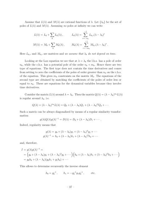
Assume that L(λ) and M(λ) are rational functions of λ. Let {λ k } be the set of
poles of L(λ) and M(λ). Assuming no poles at infinity we can write
L(λ) = L 0 + ∑ k
M(λ) = M 0 + ∑ k
L k (λ) , L k (λ) =
M k (λ) , M k (λ) =
∑−1
r=−n k
L k,r (λ − λ k ) r
∑−1
r=−m k
M k,r (λ − λ k ) r .
Here L k,r and M k,r are matrices and we assume that λ k do not depend on time.
Looking at the Lax equation we see that at λ = λ k the l.h.s. has a pole of order
n k , while the r.h.s. has a potential pole of the order n k + m k . Hence there are two
type of equations. The first type does not contain the time derivatives and comes
from setting to zero the coefficients of the poles of order greater than n k on the r.h.s.
of the equation. This gives m k constraints on the matrix M k . The equations of the
second type are obtained by matching the coefficients of the poles of order less or
equal to n k . These are equations for the dynamical variables because they involve
time derivatives.
Consider the matrix L(λ) around λ = λ k . Then the matrix Q(λ) = (λ − λ k ) n k L(λ)
is regular around λ k , i.e.
Q(λ) = (λ − λ k ) n k
L(λ) = Q 0 + (λ − λ k )Q 1 + (λ − λ k ) 2 Q 2 + · · ·
Such a matrix can be always diagonalized by means of a regular similarity transformation
g(λ)Q(λ)g(λ) −1 = D(λ) = D 0 + (λ − λ k )D 1 + · · · .
Indeed, regularity means that
and, therefore,
g(λ) = g 0 + (λ − λ k )g 1 + (λ − λ k ) 2 g 2 + · · ·
g(λ) −1 = h 0 + (λ − λ k )h 1 + (λ − λ k ) 2 h 2 + · · ·
I = g(λ)g(λ) −1 =
(
)(
)
= g 0 + (λ − λ k )g 1 + (λ − λ k ) 2 g 2 + · · · h 0 + (λ − λ k )h 1 + (λ − λ k ) 2 h 2 + · · ·
= g 0 h 0 + (λ − λ k )(g 0 h 1 + g 1 h 0 ) + · · ·
This allows to determine recurrently the inverse element
h 0 = g −1
0 , h 1 = −g −1
0 g 1 g −1
0 , etc.
– 37 –