Student Seminar: Classical and Quantum Integrable Systems

Thus, p(λ) is the generating function for the commuting local conserved quantities
The first three integrals are
I 0 = i
4s
I n =
∫ 2π
0
∫ 2π
I 1 = − 1
16s 3 ∫ 2π
I 2 =
0
dx ρ n (x) .
( S+
)
dx log ∂ x S 3 ,
S −
0
i ∫ 2π
64s 5
0
(
dx tr ∂ x S∂ x S
)
,
( )
dx tr S[∂ x S, ∂xS]
2 .
The integrals I 0 and I 1 correspond to momentum and energy respectively.
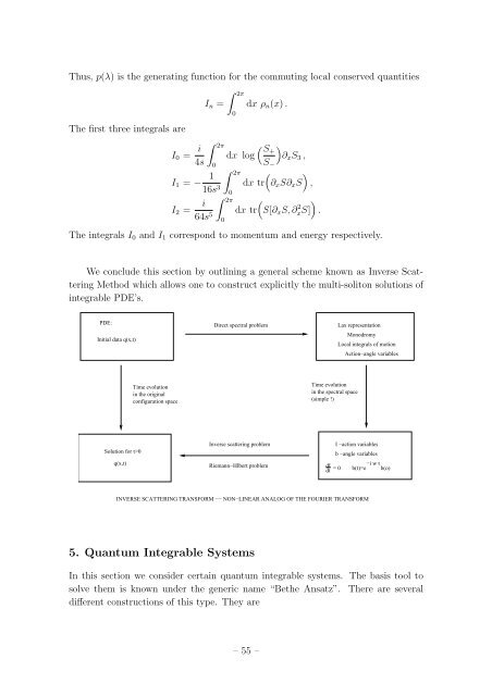
We conclude this section by outlining a general scheme known as Inverse Scattering
Method which allows one to construct explicitly the multi-soliton solutions of
integrable PDE’s.
PDE:
Initial data q(x,t)
Direct spectral problem
Lax representation
Monodromy
Local integrals of motion
Action−angle variables
Time evolution
in the original
configuration space
Time evolution
in the spectral space
(simple !)
Solution for t>0
q(x,t)
Inverse scattering problem
Riemann−Hlbert problem
dI
dt = 0
I −action variables
b −angle variables
b(t)=e−i
w t b(o)
INVERSE SCATTERING TRANSFORM −− NON−LINEAR ANALOG OF THE FOURIER TRANSFORM
5. Quantum Integrable Systems
In this section we consider certain quantum integrable systems. The basis tool to
solve them is known under the generic name “Bethe Ansatz”. There are several
different constructions of this type. They are
– 55 –