Quantile/expectile regression, and extreme data analysis

Quantile/expectile regression, and extreme data
analysis
© T. W. Yee
University of Auckland
18 July 2012 @ Cagliari
t.yee@auckland.ac.nz
http://www.stat.auckland.ac.nz/~yee
© T. W. Yee (University of Auckland) Quantile/expectile regression, and extreme data analysis 18 July 2012 @ Cagliari 1/101 1 / 101

Outline of this document
Outline of this document
1 LMS quantile regression
2 Expectile regression
3 Asymmetric MLE
4 Asymmetric Laplace distribution
5 Extreme value data analysis
6 Concluding remarks
© T. W. Yee (University of Auckland) Quantile/expectile regression, and extreme data analysis 18 July 2012 @ Cagliari 2/101 2 / 101

LMS quantile regression
Introduction to quantile regression I
Some motivation
Q: Why quantile regression?
A: Because
there is no information loss: cdf F contains all the information about
a random variable,
sometimes the tails are of more interest than in the central area.
Applications of quantile regression come from many fields. Here are
some.
Medical examples include investigating height, weight, body mass
index (BMI) as a function of age of the person. Historically, the
construction of ‘growth charts’ was probably the first example of
age-related reference intervals. Another example is Campbell and
Newman (1971)—the ultrasonographic assessment of fetal growth has
become clinically routine.
© T. W. Yee (University of Auckland) Quantile/expectile regression, and extreme data analysis 18 July 2012 @ Cagliari 3/101 3 / 101

LMS quantile regression
Introduction to quantile regression II
Some motivation
Economics, e.g., it has been used to study determinants of wages,
discrimination effects, and trends in income inequality. See
Koenker (2005) for more references.
Education, e.g., the performance of students in public schools on
standardized exams as a function of socio-economic variables such as
parents’ income and educational attainment.
Climate data, e.g., the Melbourne temperature data exhibits bimodal
behaviour.
© T. W. Yee (University of Auckland) Quantile/expectile regression, and extreme data analysis 18 July 2012 @ Cagliari 4/101 4 / 101

LMS quantile regression
Introduction to quantile regression III
Some motivation
40
Today's Max Temperature
30
20
10
10 20 30 40
Yesterday's Max Temperature
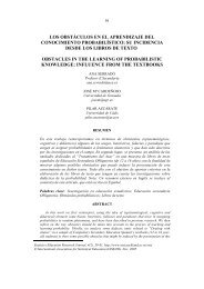
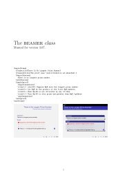
Figure: Melbourne temperature data ( ◦ C). These are daily maximum
temperatures during 1981–1990, n = 3650. Y = each day’s maximum
temperature, X = the previous day’s maximum temperature.
© T. W. Yee (University of Auckland) Quantile/expectile regression, and extreme data analysis 18 July 2012 @ Cagliari 5/101 5 / 101

LMS quantile regression
Introduction to quantile regression IV
Some motivation
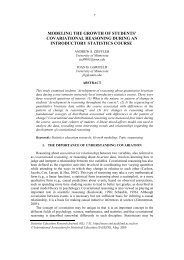
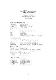
Figure: Map of Australia.
© T. W. Yee (University of Auckland) Quantile/expectile regression, and extreme data analysis 18 July 2012 @ Cagliari 6/101 6 / 101

LMS quantile regression
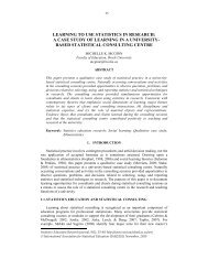
Growth chart example
Boys’ height.
© T. W. Yee (University of Auckland) Quantile/expectile regression, and extreme data analysis 18 July 2012 @ Cagliari 7/101 7 / 101

LMS quantile regression
Growth chart example
Girls’ height and weight.
© T. W. Yee (University of Auckland) Quantile/expectile regression, and extreme data analysis 18 July 2012 @ Cagliari 8/101 8 / 101

LMS quantile regression
Three subclasses I
The R package VGAM implements 3 subclasses of models for
quantile/expectile regression.
1 LMS-type methods. These transform the response to some
parametric distribution (e.g., Box-Cox to N(0, 1)). Estimated
quantiles on the transformed scale are back-transformed on to the
original scale Cole and Green (1992).
2 Expectile regression methods. If quantiles can be described as being
based on first-order moments then expectiles are second-order
moments.
3 Asymmetric Laplace distribution (ALD) models. These exploit the
property that the MLE of the location parameter of an ALD
corresponds to the classical quantile regression estimator Koenker and
Bassett (1978).
© T. W. Yee (University of Auckland) Quantile/expectile regression, and extreme data analysis 18 July 2012 @ Cagliari 9/101 9 / 101

LMS quantile regression
LMS quantile regression I
First method: the Cole-Green method
Will use an approximate random sample of 700 adults. 18 ≤ age ≤ 85.
Y = Body Mass Index (BMI; weight ÷ height 2 , kg m −2 ), a measure of
obesity.
60
●
●
50
●
●
BMI
40
30
20
●
●
●
● ●
●
●
● ●
●
● ● ●●
●
●
●
●
●
●●
● ●
● ●
●
●
● ● ●
● ●
● ●
● ●●
● ●
●
● ●
●
●
●
●
●
● ● ● ●
●
●
●
●
●
●
● ●
● ●
●
●
●
● ●
● ●●
●
●
●
●
●
●
●
●
●
●
●
●
●
●
●
●
●
●
●
● ●
●
●
● ●
●
●
●
●
● ●
●
●
●
●
●
●
●
● ●
●
●
● ●
●
●
● ●
●
●
● ●
●
●
●
●
● ●
●
●
●
● ●
●
●
●
●
●
●
●
●
●
●
●● ●
●
●
●
●
●
●
●
●
● ●
●
●
●
●
● ●
●
● ●
●
●
●
●
●
● ●
●
● ●
●
● ●
●
●
●
●
●
●
●
●
●
●
●
●
● ●
●
● ● ●
●
●
●
●
●
●●
●
●
●
●
●
●
●
●
●
●
●
●
●
●
●
●
●
●
● ●
●
●
●
●
●
●
●
●
●
●
●
●
●
●
●
●
●
●
●
● ● ●
●
●
●●
●
●
●
● ●
●
●
● ● ●
●
●
● ●
● ●
●
●
●
●
●
●
●
● ●
●
●
●
● ●
●
●
●
●
●● ●
●
●
●
●
●
●
●
●
● ●● ● ● ●
● ●
● ●
●
●
●
●
●
●
●
●
●
●
●
●
● ● ●
●
●
●
● ●
●
●
20 30 40 50 60 70 80
age
© T. W. Yee (University of Auckland) Quantile/expectile regression, and extreme data analysis 18 July 2012 @ Cagliari 10/101/ 101

LMS quantile regression
LMS quantile regression II
First method: the Cole-Green method
For scatterplot data (x i , y i ), the LMS method assumes a Box-Cox power
transformation of the y i , given x i , is standard normal. That is,
⎧
( Y
Z =
⎪⎨
⎪⎩
) λ(x)
− 1
µ(x)
σ(x) λ(x)
( )
1 Y
σ(x) log µ(x)
, λ(x) ≠ 0;
, λ(x) = 0,
(1)
is N(0, 1). “LMS” ≡ λ, µ, σ. Because σ > 0, default is
η(x) = (λ(x), µ(x), log(σ(x))) T .
© T. W. Yee (University of Auckland) Quantile/expectile regression, and extreme data analysis 18 July 2012 @ Cagliari 11/101/ 101

LMS quantile regression
LMS quantile regression III
First method: the Cole-Green method
Given ̂η, the 100α% quantile (e.g., α = 50 for median) is
[
̂µ(x) 1 + ̂λ(x)
1/ λ(x)
̂σ(x) Φ (α/100)] −1 b
. (2)
i.e., apply the inverse Box-Cox transformation to N(0, 1) quantiles. Easy!
A problem with the LMS method is to find justification for the underlying
method.
© T. W. Yee (University of Auckland) Quantile/expectile regression, and extreme data analysis 18 July 2012 @ Cagliari 12/101/ 101

LMS quantile regression
Using the gamma model avoids a range of problems:
It has finite expectations of the required derivatives of the likelihood
function (not so for the normal version, particularly when σ is small.)
The off-diagonal elements of the W i are 0 (or ≈ 0) (relative to the
diagonal elts).
Unlike the normal case, the range of transformation does not depend
on λ. Thus, in the gamma model Y ranges over (0, ∞) for all λ, µ
and σ.
© T. W. Yee (University of Auckland) Quantile/expectile regression, and extreme data analysis 18 July 2012 @ Cagliari 13/101/ 101
Second Method: The LMS Gamma Method†
Lopatatzidis and Green (1998) proposed transforming Y to a gamma
distribution—it has some theoretical and practical advantages. Then
W
= (Y /µ) λ
is assumed gamma with unit mean and variance λ 2 σ 2 . The 100α percentile
of Y at x is µ(x) Wα
1/λ(x) where W α is the equivalent deviate of size α for
the gamma distribution with mean 1 and variance λ(x) 2 σ(x) 2 .

LMS quantile regression
Third Method: The Yeo-Johnson transformation† I
Yeo and Johnson (2000) introduce a new power transformation which is
well defined on the whole real line, and potentially useful for improving
normality:
ψ(λ, y) =
⎧
⎪⎨
⎪⎩
λ = 1 = the identity transformation.
(y + 1) λ − 1
(y ≥ 0, λ ≠ 0),
λ
log(y + 1) (y ≥ 0, λ = 0),
− (−y + 1)2−λ − 1
(y < 0, λ ≠ 2),
2 − λ
− log(−y + 1) (y < 0, λ = 2).
The Yeo-Johnson transformation is equivalent to the generalized Box-Cox
transformation for y > −1 where the shift constant 1 is included.
© T. W. Yee (University of Auckland) Quantile/expectile regression, and extreme data analysis 18 July 2012 @ Cagliari 14/101/ 101

LMS quantile regression
Box−Cox transformation of y
3
2
1
0
−1
−2
−5
−3
0
1
3
5
−3
−3 −2 −1 0 1 2 3
y
Figure: The Box-Cox transformation (y λ − 1)/λ.
© T. W. Yee (University of Auckland) Quantile/expectile regression, and extreme data analysis 18 July 2012 @ Cagliari 15/101/ 101

LMS quantile regression
Yeo−Johnson transformation of y
3
2
1
0
−1
−2
−5
−3
0
1
3
5
−3
−3 −2 −1 0 1 2 3
y
Figure: The Yeo-Johnson transformation ψ(λ, y).
© T. W. Yee (University of Auckland) Quantile/expectile regression, and extreme data analysis 18 July 2012 @ Cagliari 16/101/ 101

LMS quantile regression
VGAM software for quantile/expectile regression
VGAM family functions for quantile/expectile regression.
lms.bcn() Box-Cox transformation to normality
lms.bcg() Box-Cox transformation to gamma distribution
lms.yjn() Yeo-Johnson transformation to normality
amlnormal() Asymmetric least squares
amlbinomial() Asymmetric maximum likelihood—for binomial
amlpoisson() Asymmetric maximum likelihood—for Poisson
amlexponential() Asymmetric maximum likelihood—for exponential
alaplace1() AL ∗ (ξ) with known σ, and κ (or τ)
alaplace2() AL ∗ (ξ, σ) with known κ (or τ)
alaplace3() AL ∗ (ξ, σ, κ)
© T. W. Yee (University of Auckland) Quantile/expectile regression, and extreme data analysis 18 July 2012 @ Cagliari 17/101/ 101

LMS quantile regression
lms. functions I
> args(lms.bcn)
function (percentiles = c(25, 50, 75), zero = c(1, 3), llambda = "identity",
lmu = "identity", lsigma = "loge", elambda = list(), emu = list(),
esigma = list(), dfmu.init = 4, dfsigma.init = 2, ilambda = 1,
isigma = NULL, expectiles = FALSE)
NULL
> args(lms.bcg)
function (percentiles = c(25, 50, 75), zero = c(1, 3), llambda = "identity",
lmu = "identity", lsigma = "loge", elambda = list(), emu = list(),
esigma = list(), dfmu.init = 4, dfsigma.init = 2, ilambda = 1,
isigma = NULL)
NULL
> args(lms.yjn)
function (percentiles = c(25, 50, 75), zero = c(1, 3), llambda = "identity",
lsigma = "loge", elambda = list(), esigma = list(), dfmu.init = 4,
dfsigma.init = 2, ilambda = 1, isigma = NULL, rule = c(10,
5), yoffset = NULL, diagW = FALSE, iters.diagW = 6)
NULL
© T. W. Yee (University of Auckland) Quantile/expectile regression, and extreme data analysis 18 July 2012 @ Cagliari 18/101/ 101

LMS quantile regression
Cole and Green (1992) advocated estimation by penalized likelihood using
splines. Their penalized log-likelihood was
n∑
l i − 1 2 λ λ
i=1
which is a special case of
∫ {λ ′′ (t) } ∫
2 1 {µ
dt −
2 λ µ
′′ (t) } ∫
2 1 {σ
dt −
2 λ σ
′′ (t) } 2 dt,
n∑
i=1
l i − 1 2
p∑
M∑
k=1 j=1
λ (j)k
∫ {
f ′′
(j)k (x k)} 2
dxk . (3)
This is exactly the VGAM framework!
Of the three functions, it is often a good idea to allow µ(x) to be more
flexible and/or set λ and σ to be an intercept term only, e.g., s(x2, df =
c(1, 4, 1)) or lms.bcn(zero = c(1, 3)).
© T. W. Yee (University of Auckland) Quantile/expectile regression, and extreme data analysis 18 July 2012 @ Cagliari 19/101/ 101

LMS quantile regression
Example with bmi.nz I
> fit = vgam(BMI ~ s(age, df = c(1, 4, 1)), trace = FALSE,
fam = lms.bcn(zero = NULL), bmi.nz)
> qtplot(fit, pcol = "blue", tcol = "orange", lcol = "orange")
20 30 40 50 60 70 80 90
20
30
40
50
60
age
●
●
●
●
●
●
●
●
●
●
●
●
●
●
●
●
●
●
●
●
●
●
●
●
●
●
●
●
●
●
●
●
●
●
●
●
●
●
●
●
●
●
●
●
●
●
●
●
●
●
●
●
●
●
●
●
●
●
●
●
●
●
●
●
●
●
●
●
●
●
●
●
●
●
●
●
●
●
●
●● ●
●
●
●
●
●
●
●
●
●
●
●
●
●
● ● ●
●
●
●
●
●
●
●
●
●
●
●
●
●
●
●
●
●
●
●
●
●
●
●●
●
●
●
●
●
●
●
●
●
●
●
●
●
●
●
●
●
●
●
●
●
●
●
●
●
●
●
●
●
●
●
●
●
●
●
●
●
●
●
●
●
●
●
●
●
●
●
●
●
●
●
●
●
●
●
●
●
●
●
●
●
●
●
●
●
●
●
●
●
●
●
●
●
●
●
●
●
●
●
●
●
●
●
●
●
●
●
●
●
●
●
●
●
●
●
●
●
●
●
●
●
●
●
●
●
●
●
●
●
●
●
●
●
●
●
●
●
●
●
●
●
●
●
●
●
●
●
●
●
●
●
●
●
●
●
●
●
●
●
●
●
●
●
●
●
●
●
●
●
●
●
●
●
●
●
●
●
●
●
●
●
●
●
●
●
●
●
●
●
●
●
●
●
●
●
●
●
●
●
●
●
●
●
●
●
●
●
●
●
●
●
●
●
●
●
●
●
●
●
●
●
●
●
●
●
●
●
●
●
●
●
●
●
●
●
● ●
●
●
●
●
●
●
●
●
●
●
●
●
●
●
●
●
●
●
●
●
●
●
●
●
●
● ●
●
●
●
●
●
●
●
●
●
●
●
●
●
●
●
●
●
●
●
●
●
●
●
●
●
●
●
●
●
●
●
●
●
●
●
●
●
●
●
●
●
●
●
●
●
●
●
●
●
●
●
●
●
●
●
●
●
●
●
●
●
●
●
●
●
●
●
●
●
●
●
●
●
●
●
●
●
●
●
●
●
●
●
●
●
●
●
●
●
●
●
●
●
●
●
●
●
●
●
●
●
●
●
●
●
●
●
●
●
●
●
●
●
●
●
●
●
●
●
●
●
●
●
●
●
●
●
●
●
●
●
●
●
●
●
●
●
●
●
●
●
●
●
●
●
●
●
●
●
●
●
●
●
●
●
●
●
●
●
●
●
●
●
●
●
●
●
●
●
●
●
●
●
●
●
●
●
●
●
●
●
●
●
●
●
●
●
●
● ●
●
●
●
●
●
●
●
●
●
●
●
●
●
●
●
●
●
●
●
●
●
●
●
●
●
●
●
●
●
●
●
●
●
●
●
●
●
●
●
●
●
●
●
●
●
●
●
●
●
●
●
●
●
●
●
●
●
●
●
●
●
●
●
●
●
●
●
●
●
●
●
●
●
●
●
●
●
●
●
●
●
●
●
●
●
●
●
●
●
●
●
●
●
●
●
●
●
●
●
●
●
●
●
●
●
●
●
●
●
●
●
●
●
●
●
●
●
●
●
●
●
● ●
●
●
●
●
●
●
●
●
●
●
●
●
●
●
●
●
●
●
●
●
●
25%
50%
75%
© T. W. Yee (University of Auckland) Quantile/expectile regression, and extreme data analysis 20/101
18 July 2012 @ Cagliari 20 / 101

LMS quantile regression
Example with bmi.nz II
Q: Why the decrease at older years?
A:
© T. W. Yee (University of Auckland) Quantile/expectile regression, and extreme data analysis 18 July 2012 @ Cagliari 21/101/ 101

LMS quantile regression
Example with bmi.nz III
Q: Why the decrease at older years?
A: Selection bias due to premature death of obese people.
© T. W. Yee (University of Auckland) Quantile/expectile regression, and extreme data analysis 18 July 2012 @ Cagliari 22/101/

LMS quantile regression
Example with bmi.nz IV
> ygrid = seq(15, 43, len = 100) # BMI ranges
> mycols aa = deplot(fit, x0 = 20, y = ygrid, xlab = "BMI", col = mycols[1],
main = "Estimated density functions")
> aa = deplot(fit, x0 = 42, y = ygrid, add = TRUE,
col = mycols[2])
> aa = deplot(fit, x0 = 55, y = ygrid, add = TRUE,
col = mycols[3], Attach = TRUE)
> legend("topright", col = mycols, lty = 1,
c("20 year olds", "42 year olds", "55 year olds"))
© T. W. Yee (University of Auckland) Quantile/expectile regression, and extreme data analysis 18 July 2012 @ Cagliari 23/101/

LMS quantile regression
Example with bmi.nz V
Estimated density functions
0.10
20 year olds
42 year olds
55 year olds
0.08
density
0.06
0.04
0.02
0.00
15 20 25 30 35 40
BMI
Figure: Density plot at various ages.
© T. W. Yee (University of Auckland) Quantile/expectile regression, and extreme data analysis 18 July 2012 @ Cagliari 24/101/

LMS quantile regression
Example with bmi.nz VI
> aa@post$deplot # Contains density function values
$newdata
age
1 55
$y
[1] 15.00 15.28 15.57 15.85 16.13 16.41 16.70 16.98 17.26
[10] 17.55 17.83 18.11 18.39 18.68 18.96 19.24 19.53 19.81
[19] 20.09 20.37 20.66 20.94 21.22 21.51 21.79 22.07 22.35
[28] 22.64 22.92 23.20 23.48 23.77 24.05 24.33 24.62 24.90
[37] 25.18 25.46 25.75 26.03 26.31 26.60 26.88 27.16 27.44
[46] 27.73 28.01 28.29 28.58 28.86 29.14 29.42 29.71 29.99
[55] 30.27 30.56 30.84 31.12 31.40 31.69 31.97 32.25 32.54
[64] 32.82 33.10 33.38 33.67 33.95 34.23 34.52 34.80 35.08
[73] 35.36 35.65 35.93 36.21 36.49 36.78 37.06 37.34 37.63
[82] 37.91 38.19 38.47 38.76 39.04 39.32 39.61 39.89 40.17
[91] 40.45 40.74 41.02 41.30 41.59 41.87 42.15 42.43 42.72
[100] 43.00
$density
[1] 4.589e-05 7.826e-05 1.293e-04 2.076e-04 3.240e-04
© T. W. Yee (University of Auckland) Quantile/expectile regression, and extreme data analysis 18 July 2012 @ Cagliari 25/101/

LMS quantile regression
Example with bmi.nz VII
[6] 4.927e-04 7.308e-04 1.059e-03 1.501e-03 2.083e-03
[11] 2.835e-03 3.785e-03 4.965e-03 6.403e-03 8.125e-03
[16] 1.016e-02 1.251e-02 1.520e-02 1.822e-02 2.157e-02
[21] 2.524e-02 2.920e-02 3.341e-02 3.783e-02 4.242e-02
[26] 4.712e-02 5.188e-02 5.662e-02 6.129e-02 6.582e-02
[31] 7.016e-02 7.425e-02 7.803e-02 8.147e-02 8.453e-02
[36] 8.717e-02 8.937e-02 9.112e-02 9.241e-02 9.324e-02
[41] 9.362e-02 9.356e-02 9.307e-02 9.219e-02 9.094e-02
[46] 8.935e-02 8.745e-02 8.528e-02 8.286e-02 8.024e-02
[51] 7.745e-02 7.452e-02 7.149e-02 6.838e-02 6.523e-02
[56] 6.205e-02 5.888e-02 5.573e-02 5.262e-02 4.957e-02
[61] 4.660e-02 4.371e-02 4.092e-02 3.823e-02 3.564e-02
[66] 3.318e-02 3.083e-02 2.860e-02 2.648e-02 2.449e-02
[71] 2.261e-02 2.084e-02 1.919e-02 1.764e-02 1.620e-02
[76] 1.486e-02 1.361e-02 1.245e-02 1.138e-02 1.039e-02
[81] 9.480e-03 8.638e-03 7.864e-03 7.152e-03 6.500e-03
[86] 5.902e-03 5.355e-03 4.854e-03 4.398e-03 3.981e-03
[91] 3.601e-03 3.256e-03 2.942e-03 2.656e-03 2.397e-03
[96] 2.162e-03 1.949e-03 1.756e-03 1.582e-03 1.424e-03
© T. W. Yee (University of Auckland) Quantile/expectile regression, and extreme data analysis 18 July 2012 @ Cagliari 26/101/

LMS quantile regression
Example with bmi.nz VIII
Two general quantile regression problems
1 Most methods cannot handle count data, proportions, etc.
Q: LMS-quantile regression won’t handle the Melbourne temperature
data. Why?
A:
2 Some methods suffer from the “serious embarrassment” 1 of quantile
crossing, e.g., a point (x 0 , y 0 ) may be classified as below the 20th but
above the 30th percentile!
1 see, e.g., He (1997), Sec. 2.5 of Koenker (2005).
© T. W. Yee (University of Auckland) Quantile/expectile regression, and extreme data analysis 18 July 2012 @ Cagliari 27/101/

LMS quantile regression
Two quantile regression problems
oooooo oooo
o
o
o
ooo
o
o
o
oo
o
oo
o
o
o
oo
o
o
o
o
o
o
o
o
o
o
o
o
oo
o
o
oo
o
o
oo
o
o
oo
o
o
o
o
o
o
o
o
o
o
o
o
o
o
o
o
o
o
o
o
o
o
o
o
o
o
o
o
o
oo
o
o
o
o
o
o
o
o
o
o
o
o
o
o
o
o
o
o
o
o
o
o
o
o
o
o
o
o
o
o
o
o
o
o
o
o
o
o
o
o
o
o
o
o
o
o
o
o
o
o
o
o
o
o
o
o
o
o
o
o
o
oo
o
o
o
o
o
o
o
o
o
o
o
o
o
o
o
o
o
o
o
o
o
o
o
o
o
o
o
o
o
o
o
o
o
o
o
o
o
o
o
o
o
o
o
o
o
o
o
o
o
o
o
o
o
o
o
o
o
o
o
o
o
o
o
o
o
o
o
o
o
o
o
o
o
o
o
o
o
o
o
o
o
o
o
o
o
o
o
o
o
o
oo
o
o
o
o
o
o
o
o
o
o
o
o
oo
o
o
o
o
o
o
o
o
o
o
o
o
o
o
o
o
o
o
o
o
o
o
o
o
o
o
o
o
o
o
o
o
o
o
o
o
o
o
o
o
o
o
o
o
o
o
o
o
o
o
o
o
o
o
o
o
o
o
o
o
o
o
o
o
oo
o
o
o
o
o
o
o
o
o
o
o
oo
o
o
o
o
o
o
o
o
o
o
o
o
o
o
o
o
o
o
o
o
o
oo
o
o
oo
o
o
o
o
o
o
o
o
o o o
o
o
o
oo
o
o
o
o
o
o
o
o
o
o
oo
o
o
o
o
o
oo
o
o
o
o
o
o
o
o
o
o
o
o
o
o
o
o
o
o
o
o
o
o
o
o
o
o
o
o
o
0.0 0.2 0.4 0.6 0.8 1.0
0
5
10
15
x
y
Some Poisson data.
© T. W. Yee (University of Auckland) Quantile/expectile regression, and extreme data analysis 28/101
18 July 2012 @ Cagliari 28 / 101

LMS quantile regression
Some Poisson data with 50 and 95 percentiles from qpois().
© T. W. Yee (University of Auckland) Quantile/expectile regression, and extreme data analysis 18 July 2012 @ Cagliari 29/101/ Two quantile regression problems
y
15
10
5
0
o
o
o o
o
o
o o
o
ooo
o o o
o
o
o o o o o o o o
o oo
o
o
o oo
o oo
o o
o o o
o
o o o o oo o oo
o
o
o oo
o o
o o o o o
o o
oo
o o o o o
o o
o o o o
o
o oo
oo
oo
o o o o
o
o
oo
o
o o
o o o
o oo
o
o o o oo
o o o o
o
o oo
o
o o o oo
oo
o
oo
oo
o o o o
o o o
o o
o o o o ooo
o o
o o o
o o
oo
oo
o oo
oo o o o o
o o
o o o o oo o o o
o
oo
o
o oo
o
o
o o
o
o o
o oo
o o o
o o o o
o
o o o
o o o o o o
o
o oo oo oo oo
o
o
o o o
o
o
ooo
o o o
ooo
o
o o o o o
o o o
o
o o o o o ooo
o
o
o
oo
o o
oo
o ooo
o o
o o o oo
oo
oo o
o
oo
oooooo oooo oooo
ooo
oo
ooo
ooo
ooo
o
o
o
oo
o ooo
o
0.0 0.2 0.4 0.6 0.8 1.0
x

Expectile regression
Expectile regression
Quantiles:
minimize wrt ξ the quantity E [ρ τ (Y − ξ)] where
ρ τ (u) = u · (τ − I (u < 0)), 0 < τ < 1, (4)
is known as a check function. I call this the “classical” method Koenker
and Bassett (1978). See package quantreg.
Expectiles:
[ ]
minimize wrt µ the quantity E ρ [2]
ω (Y − µ) where
ρ [2]
ω (u) = u 2 · |ω − I (u < 0)|, 0 < ω < 1. (5)
© T. W. Yee (University of Auckland) Quantile/expectile regression, and extreme data analysis 18 July 2012 @ Cagliari 30/101/

Expectile regression
Interpretation I
Both have very natural interpretations: given X = x,
quantile ξ τ (x) specifies the position below which 100τ% of the
(probability) mass of Y lies.
expectile µ ω (x) determines the point such that 100ω% of the mean
distance between it and Y comes from the mass below it.
The 0.5-expectile µ( 1 2
) is the mean µ.
The 0.5-quantile ξ( 1 2
) is the median ˜µ.
Quantiles are more local whereas expectiles are more global and are
affected by outliers.
Quantiles traditionally are estimated by linear programming whereas
expectiles use scoring.
© T. W. Yee (University of Auckland) Quantile/expectile regression, and extreme data analysis 18 July 2012 @ Cagliari 31/101/ 101

Expectile regression
Interpretation II
2.0
ω = 0.5
ω = 0.9
(a)
2.0
(b)
1.5
1.5
Loss
1.0
1.0
0.5
0.5
0.0
0.0
−2 −1 0 1 2
−2 −1 0 1 2
Figure: Loss functions for (a) quantile regression with τ = 0.5 (L 1 regression) and
τ = 0.9; (b) expectile regression with ω = 0.5 (least squares) and ω = 0.9.
(a) are aka asymmetric absolute loss function or pinball loss function.
© T. W. Yee (University of Auckland) Quantile/expectile regression, and extreme data analysis 18 July 2012 @ Cagliari 32/101/

Expectile regression
Expectiles I
Expectiles and centers of balance
(d)
c 1 c 2
µ(ω = 0.1)
Figure: Illustration of the interpretation of expectiles in terms of centers of
balance, at positions c 1 = △ and c 2 = △. This means that (6) is satisfied
with ω = 0.1. Note: the parent distribution is normal.
© T. W. Yee (University of Auckland) Quantile/expectile regression, and extreme data analysis 18 July 2012 @ Cagliari 33/101/

Expectile regression
Expectiles II
Expectiles and centers of balance
Even simpler interpretation is via centers of balance. From Slide 33, c 1
and c 2 denote the centers of balance for the distributions to the LHS and
RHS of the ω-expectile µ(ω). Then
ω =
P[Y < µ(ω)] · (µ(ω) − c 1 )
P[Y < µ(ω)] · (µ(ω) − c 1 ) + P[Y > µ(ω)] · (c 2 − µ(ω))
where c 1 = E[Y |Y < µ(ω)] =
is a fundamental equation. If µ(ω) = 0 then
∫ µ(ω)
−∞
y
[ ] f (y)
dy
F (µ(ω))
(6)
ω =
|c 1 | · F (0)
|c 1 | · F (0) + c 2 · (1 − F (0)) .
© T. W. Yee (University of Auckland) Quantile/expectile regression, and extreme data analysis 18 July 2012 @ Cagliari 34/101/

Expectile regression
Expectiles III
Expectiles and centers of balance
Another fundamental equation is
µ = µ(0.5) = P[Y < µ(ω)] · c 1 + P[Y > µ(ω)] · c 2 . (7)
BTW c 1 is related to the expected shortfall, which is used in financial
mathematics—see Slide 40.
© T. W. Yee (University of Auckland) Quantile/expectile regression, and extreme data analysis 18 July 2012 @ Cagliari 35/101/

Expectile regression
Interrelationship between expectiles and quantiles† I
“Expectiles have properties that are similar to quantiles” (Newey and
Powell, 1987). The reason is that expectiles of a distribution F are
quantiles a distribution G which is related to F (Jones, 1994).
The main details are as follows.
Let
P(s) =
∫ s
−∞
y f (y) dy
ρ [1]
τ (u) = τ − I (u ≤ 0),
ρ [2]
ω (u) = |u|(ω − I (u < 0)).
the (first) partial moment,
© T. W. Yee (University of Auckland) Quantile/expectile regression, and extreme data analysis 18 July 2012 @ Cagliari 36/101/

Expectile regression
Interrelationship between expectiles and quantiles† II
One way of defining the ordinary τ-quantile of a continuous distribution
with density f , 0 < τ < 1, is as the value of ξ that satisfies
∫
ρ [1]
τ (y − ξ) f (y) dy = 0.
In a similar way, for expectiles µ(ω), corresponds to the equation
∫
ρ [2]
ω (y − µ(ω)) f (y) dy = 0. (8)
Then solving this equation shows immediately that ω = G(µ(ω)) where
G(t) =
P(t) − tF (t)
2(P(t) − tF (t)) + t − µ . (9)
© T. W. Yee (University of Auckland) Quantile/expectile regression, and extreme data analysis 18 July 2012 @ Cagliari 37/101/

Expectile regression
Interrelationship between expectiles and quantiles† III
Thus, G is the inverse of the expectile function, and its derivative is
g(t) =
µF (t) − P(t)
{2(P(t) − tF (t)) + t − µ} 2 . (10)
It can be shown that G is actually a distribution function (so that g is its
density function). That is, the expectiles of F are precisely the quantiles
of G defined here.
Table: Density function, distribution function, and expectile function and random
generation for the distribution associated with the expectiles of several
standardized distributions. These functions are available in VGAM.
Function
[dpqr]eexp()
[dpqr]ekoenker()
[dpqr]enorm()
[dpqr]eunif()
Distribution
Exponential
Koenker
Normal
Uniform
© T. W. Yee (University of Auckland) Quantile/expectile regression, and extreme data analysis 18 July 2012 @ Cagliari 38/101/

Expectile regression
Interrelationship between expectiles and quantiles† IV
0.6
(a) Normal
2.0
(b) Uniform
0.5
0.4
0.3
1.5
1.0
0.2
0.1
0.5
0.0
0.0
−4 −2 0 2 4
0.0 0.2 0.4 0.6 0.8 1.0
1.0
(c) Exponential
0.4
(d) Koenker
0.8
0.3
0.6
0.4
0.2
0.2
0.1
0.0
0.0
0 1 2 3 4 5
−4 −2 0 2 4
Figure: (a)–(c) Density plots of expectile g (purple solid lines) for the original f
of standard normal, uniform and exponential distributions (blue dashed lines);
(d) Koenker’s distribution is the same as a √ 2 T 2 density. Orange line is N(0, 1).
© T. W. Yee (University of Auckland) Quantile/expectile regression, and extreme data analysis 18 July 2012 @ Cagliari 39/101/

Expectile regression
Expected shortfall† I
Value at Risk
The expected shortfall (ES) 2 is a concept used in financial mathematics
to measure portfolio risk. Aka
Conditional Value at Risk (CVaR),
expected tail loss (ETL) and
worst conditional expectation (WCE).
The ES at the 100τ% level is the expected return on the portfolio in the
worst 100τ% of the cases. It is often defined as
ES(τ) = E(Y |Y < a) (11)
where a is determined by P(X < a) = τ and τ is the given threshold.
© T. W. Yee (University of Auckland) Quantile/expectile regression, and extreme data analysis 18 July 2012 @ Cagliari 40/101/

Expectile regression
Expected shortfall† II
Value at Risk
The ES is very much related to expectiles and c 1 . That is, the
solution µ(ω) of this minimization satisfies
( 1 − 2ω
ω
)
E [(Y − µ(ω)) · I (Y < µ(ω))] = µ(ω) − E(Y ). (12)
Eqn (12) indicates that the solution µ(ω) is determined by the properties
of the expectation of the random variable Y conditional on Y
exceeding µ(ω). This suggests a link between expectiles and ES.
Eqn (12) can be rewritten
(
)
ω
ω
E [Y |Y < µ(ω)] = 1 +
µ(ω)−
E(Y ).
(1 − 2ω)F (µ(ω)) (1 − 2ω)F (µ(ω))
© T. W. Yee (University of Auckland) Quantile/expectile regression, and extreme data analysis 18 July 2012 @ Cagliari 41/101/ 101

Expectile regression
Expected shortfall† III
Value at Risk
This provides a formula for the ES of the quantile that coincides with the
ω-expectile. Referring to this as the τ-quantile, we can write F (µ(ω)) = τ
and rewrite the expression as
(
ES(τ) = 1 +
ω
(1 − 2ω) τ
)
µ(ω) −
ω
E(Y ). (13)
(1 − 2ω) τ
This equation relates the ES associated with the τ-quantile of the
distribution of Y and the ω-expectile that coincides with that quantile.
The equation is for ES in the lower tail of the distribution. The equation
for the upper tail of the distribution is produced by replacing ω and τ
with (1 − ω) and (1 − τ), respectively.
© T. W. Yee (University of Auckland) Quantile/expectile regression, and extreme data analysis 18 July 2012 @ Cagliari 42/101/

Expectile regression
Expected shortfall† IV
Value at Risk
Another popular measure of financial risk is the Value at Risk (VaR). The
VaR (ν p , say) specifies a level of excessive losses such that the probability
of a loss larger than ν p is less than p (often p = 0.01 or 0.05 is chosen).
The ES is defined as the conditional expectation of the loss given that it
exceeds the VaR.
ES “better” than VaR:
ES has but VaR lacks the sub-additivity 3 property. So the ES is an
increasingly popular risk measure in financial risk management.
VaR is not a coherent risk measure.
VaR provides no information on the extent of excessive losses other
than specifying a level that defines the excessive losses.
2 Dictionary: (i). A failure to attain a specified amount or level; a shortage.
(ii). The amount by which a supply falls short of expectation, need, or demand.
3 The sub-additivity of a risk measure means that the risk for the sum of two
independent risky events is not greater than the sum of the risks of the two events.
© T. W. Yee (University of Auckland) Quantile/expectile regression, and extreme data analysis 18 July 2012 @ Cagliari 43/101/

Asymmetric MLE
Asymmetric MLE I
Asymmetric maximum likelihood estimation allows for expectile regression
based on, essentially, any distribution. Efron (1991) developed this for the
exponential family.
Consider the linear model
Let
y i = x T i β + ε i , for i = 1, . . . , n.
r i (β) = y i − x T i β
be a residual. The asymmetric squared error loss S w (β) is
S w (β) =
n∑
Qw(r ∗ i (β)) (14)
i=1
© T. W. Yee (University of Auckland) Quantile/expectile regression, and extreme data analysis 18 July 2012 @ Cagliari 44/101/

Asymmetric MLE
Asymmetric MLE II
and Q ∗ w is the asymmetric squared error loss function
Q ∗ w(r) =
{ r 2 , r ≤ 0,
w r 2 , r > 0.
(15)
Here w is a positive constant and is related to ω by
w =
ω
1 − ω . (16)
For normally distributed responses, asymmetric least squares (ALS)
estimation is a variant of OLS estimation.
Estimation is by the Newton-Raphson algorithm. Order-2
convergence is fast and, here, reliable. See later for details.
© T. W. Yee (University of Auckland) Quantile/expectile regression, and extreme data analysis 18 July 2012 @ Cagliari 45/101/

Asymmetric MLE
Asymmetric MLE III
Notation
t Notation
Comments
Y
Response. Has mean µ, cdf F (y), pdf f (y)
Q Y (τ) = τ-quantile of Y 0 < τ < 1
ξ(τ) = ξ τ = τ-quantile Koenker and Bassett (1978), ξ( 1 ) = median
2
µ(ω) = µ ω = ω-expectile 0 < ω < 1, µ( 1 ) = µ, Newey and Powell (1987)
2
bξ(τ), bµ(ω)
Sample quantiles and expectiles
centile
Same as quantile and percentile here
regression quantile Koenker and Bassett (1978)
regression expectile Newey and Powell (1987)
regression percentile All forms of asymmetric fitting, Efron (1992)
ρ τ (u) = u · (τ − I (u < 0)) Check function corresponding to ξ(τ)
ρ [2]
ω (u) = u 2 · |ω − I (u < 0)| Check function corresponding to µ(ω)
u + = max(u, 0)
Positive part of u
u − = min(u, 0)
Negative part of u
© T. W. Yee (University of Auckland) Quantile/expectile regression, and extreme data analysis 18 July 2012 @ Cagliari 46/101/

Asymmetric MLE
ALS notes I
Here are some notes about ALS quantile regression.
Usually the user will specify some desired value of the percentile, e.g.,
75 or 95. Then the necessary value of w needs to be numerically
solved for to obtain this. One useful property is that the percentile is
a monotonic function of w, meaning one can solve for the root of a
nonlinear equation.
A rough relationship between w and the percentile 100α is available.
Let w (α) denote the value of w such that β w equals z (α) = Φ −1 (α),
the 100α standard normal percentile point. If there are no covariates
(intercept-only model) and y i are standard normal then
w (α) = 1 +
z (α)
φ ( z (α)) − (1 − α)z (α) (17)
where φ(z) is the probability density function of a standard normal.
Here are some values.
© T. W. Yee (University of Auckland) Quantile/expectile regression, and extreme data analysis 18 July 2012 @ Cagliari 47/101/

Asymmetric MLE
ALS notes II
> alpha = c(1/2, 2/3, 3/4, 0.84, 9/10, 19/20)
> zalpha = qnorm(p = alpha)
> walpha = 1 + zalpha/(dnorm(zalpha) - (1 - alpha)*zalpha)
> round(cbind(alpha, walpha), dig = 2)
alpha walpha
[1,] 0.50 1.00
[2,] 0.67 2.96
[3,] 0.75 5.52
[4,] 0.84 12.81
[5,] 0.90 28.07
[6,] 0.95 79.73
An important invariance property: if the y i are multiplied by some
constant c then the solution vector ̂β w is also multipled by c. Also, a
shift in location to y i + d means the estimated intercept (the first
element in x) increases by d too.
© T. W. Yee (University of Auckland) Quantile/expectile regression, and extreme data analysis 18 July 2012 @ Cagliari 48/101/

Asymmetric MLE
ALS notes III
ALS quantile regression is consistent for the true regression
percentiles y (α) |x in the cases where y (α) |x is linear in x. A more
general proof of this is available (Newey and Powell, 1987).
In view of the one-to-one mapping between expectiles and quantiles
Efron (1991) proposes that the τ-quantile be estimated by the
expectile for which the proportion of in-sample observations lying
below the expectile is τ. This provides justification for practitioners
who use expectile regression to perform quantile regression.
Some expectile references: Aigner et al. (1976), Newey and
Powell (1987), Efron (1991), Efron (1992), Jones (1994).
© T. W. Yee (University of Auckland) Quantile/expectile regression, and extreme data analysis 18 July 2012 @ Cagliari 49/101/

Asymmetric MLE
Example I
> ooo bmi.nz fit # Expectile plot
> plot(BMI ~ age, data = bmi.nz, col = "blue", las = 1,
main = paste(paste(round(fit@extra$percentile, dig = 1),
collapse = ", "),
"expectile curves"))
> with(bmi.nz, matlines(age, fitted(fit), col = 1:npred(fit),
lwd = 2, lty = 1))
gives
© T. W. Yee (University of Auckland) Quantile/expectile regression, and extreme data analysis 18 July 2012 @ Cagliari 50/101/

Asymmetric MLE
Example II
60
●
20.1, 56.3, 85.9 expectile curves
●
50
BMI
40
30
20
●
●
●
●
●
● ●
●
●
● ●
●
● ● ●
●●
● ●
● ●
●
●
●
●
●
●
●
● ● ●
● ●
● ●
●
● ● ● ● ●
●
●
●
●
●
● ●
● ● ● ●
●
●●
● ●●
●●
●
● ●
● ●
●
●
●
●
●
● ● ●●
●
● ●
● ●● ● ● ● ●
● ●
●
●● ●
●
● ●
●
●
●
●
● ●
●
● ● ● ●
● ●
●
●
●
●
●
●
● ● ● ● ●
● ● ● ●
●
● ●
●
● ● ● ●
● ● ●
● ●
●
●
●
● ●
● ● ●
● ● ●
● ● ●
●
●
●
●
● ●●
●
●
●
● ●
●
●
●
●
●
●
●●●
● ●●
●
●
●● ●
●
●
● ●
●
●
●
● ●●
●
● ●
●
● ●
●● ● ● ● ● ●●
● ●
● ● ●
● ●
● ●●
● ●
●
●
●
● ●
● ● ●
●
●
●● ● ● ● ●
●
● ●
●
● ●
●
●
●
●
● ●
● ● ● ●●
● ●
● ●
● ●●● ● ●
●
●
●
●
● ●
● ● ● ●
●
● ●
● ●
●
●
●
● ● ●
● ● ●●
●
● ●
●
●
●
● ● ● ● ● ●
●
●●
●
● ● ● ●
●
●
●
●
20 30 40 50 60 70 80
age
© T. W. Yee (University of Auckland) Quantile/expectile regression, and extreme data analysis 18 July 2012 @ Cagliari 51/101/ 101

Asymmetric MLE
More on AML regression†
Efron (1992) generalized ALS estimation to families in the exponential
family, and in particular, the Poisson distribution. He called this
asymmetric maximum likelihood (AML) estimation.
More generally,
S w (β) =
is minimized (cf. (14)), where
n∑
i=1
w i D w (y i , µ i (β)) (18)
D w (µ, µ ′ ) =
{ D(µ, µ ′ ) if µ ≤ µ ′ ,
w D(µ, µ ′ ) if µ > µ ′ .
(19)
Here, D is the deviance from a model in the exponential family
g η (y) =
exp(ηy − ψ(η)).
© T. W. Yee (University of Auckland) Quantile/expectile regression, and extreme data analysis 18 July 2012 @ Cagliari 52/101/

Asymmetric MLE
Estimation†
An iterative solution is required, and the Newton-Raphson algorithm is
used. In particular, for Poisson regression with the canonical (log) link,
following in from Equation (2.16) of Efron (1992),
β (a+1) = b (a) + db (a)
= b − ¨S −1¨S
w w
= (X T (WV)X) −1 X T (WV)
[
]
η + (WV) −1 Wr
(20)
are the Newton-Raphson iterations (iteration number a suppressed for
clarity). Here, r = y − µ(b),
V = diag(v 1 (b), . . . , v n (b)) = diag(µ 1 , . . . , µ n ) contains the variances
of y i and W = diag(w 1 (b), . . . , w n (b)) with w i (b) = 1 if r i (b) ≤ 0 else w.
© T. W. Yee (University of Auckland) Quantile/expectile regression, and extreme data analysis 18 July 2012 @ Cagliari 53/101/

Asymmetric MLE
AML Poisson example I
> set.seed(1234)
> mydat = data.frame(x2 = sort(runif(nn mydat = transform(mydat, y = rpois(nn, exp(0 - sin(8 * x2))))
> fit = vgam(y ~ s(x2, df = 3),
amlpoisson(w.aml = c(0.02, 0.2, 1, 5, 50)),
data = mydat)
> fit@extra
$w.aml
[1] 0.02 0.20 1.00 5.00 50.00
$M
[1] 5
$n
[1] 200
$y.names
[1] "w.aml = 0.02" "w.aml = 0.2" "w.aml = 1"
[4] "w.aml = 5" "w.aml = 50"
$individual
[1] TRUE
$percentile
© T. W. Yee (University of Auckland) Quantile/expectile regression, and extreme data analysis 18 July 2012 @ Cagliari 54/101/

Asymmetric MLE
AML Poisson example II
w.aml = 0.02 w.aml = 0.2 w.aml = 1 w.aml = 5
41.5 48.0 62.0 77.5
w.aml = 50
94.0
$deviance
w.aml = 0.02 w.aml = 0.2 w.aml = 1 w.aml = 5
23.26 99.95 219.45 391.95
w.aml = 50
666.66
Then
> plot(jitter(y) ~ x2, data = mydat,
col = "blue", las = 1, main =
paste(paste(round(fit@extra$percentile, dig = 1),
collapse = ", "),
"Poisson-AML curves"))
> with(mydat, matlines(x2, fitted(fit), lwd = 2))
gives
© T. W. Yee (University of Auckland) Quantile/expectile regression, and extreme data analysis 18 July 2012 @ Cagliari 55/101/

Asymmetric MLE
AML Poisson example III
41.5, 48, 62, 77.5, 94 Poisson−AML curves
6
●
●
●
●
jitter(y)
5
4
3
2
1
0
●
● ●●
●
●
●
● ● ● ●●
●
●
● ●
● ● ●
●
●
● ●
● ● ●
● ●
●
●
● ● ●
● ●
●
● ● ●
● ● ●● ●
● ●●●
●● ● ●
●● ●
● ● ●
●
● ●
●
●●
●
●
●
●
●
●●
● ●
●
●
●
●
●
●
●
●
●
● ●
● ● ●
●
●
● ●
●
●
●
●
●
●
● ●
●
●
●
●
●
●
●
●
●
● ●
●
●
●
●
●
●
● ● ●
●
●
●
●
●
●
●
● ●
●
●●●
●● ● ●●
●
● ● ●● ●
● ● ●
● ●●
0.0 0.2 0.4 0.6 0.8 1.0
x2
© T. W. Yee (University of Auckland) Quantile/expectile regression, and extreme data analysis 18 July 2012 @ Cagliari 56/101/

Asymmetric Laplace distribution
Asymmetric Laplace distribution
Distribution properties
The asymmetric Laplace distribution (ALD) has a density
f (y; ξ, b, τ) =
=
for −∞ < y < ∞, −∞ < ξ < ∞.
τ(1 − τ)
e −ρτ (y−ξ) (21)
b
{ (
τ(1 − τ) exp −
τ
b |y − ξ|) , y ≤ ξ,
b exp ( − 1−τ
b |y − ξ|) (22)
, y > ξ,
Here, ξ is the location parameter and b is the positive scale parameter .
The expected information matrix (EIM) is
⎛
⎞
⎜
⎝
2
− √ 8
0
σ 2 σ (1+κ 2 )
1 −(1−κ
0 2 )
σ 2 σκ(1+κ 2 )
− √ 8
σ (1+κ 2 )
−(1−κ 2 )
σκ(1+κ 2 )
1
+ 4
κ 2 (1+κ 2 ) 2
⎟
⎠ . (23)
© T. W. Yee (University of Auckland) Quantile/expectile regression, and extreme data analysis 18 July 2012 @ Cagliari 57/101/

Asymmetric Laplace distribution
VGLMs and ALD
Suppose τ = (τ 1 , τ 2 , . . . , τ L ) T are either the L values of τ of interest to
the practitioner or the L reference values of τ. Let ξ s be the corresponding
τ s th quantile, s = 1, . . . , L. VGLMs use
g 1 (ξ s (x)) = η s = β T s x, s = 1, . . . , L, (24)
where g 1 is a specified parameter link function.
Hence the classical approach has g 1 being the identity link:
ξ s = β T s x.
The central formula for us is therefore
min
β
E[ ρ τ (Y − g −1
1 (βT x))]. (25)
© T. W. Yee (University of Auckland) Quantile/expectile regression, and extreme data analysis 18 July 2012 @ Cagliari 58/101/

Asymmetric Laplace distribution
Two noncrossing solutions I
The VGLM/VGAM framework offers two solutions.
1 Use parallelism.
When a parallelism assumption is made, one must choose some
reference values of τ to estimate the regression coefficients of the
model, viz.
g 1 (ξ s (x)) = η s = β (s)1 + β T (−1) x (−1) (26)
where x (−1) is x without its first element. Here the hyperplanes differ
by a constant amount at a given value of x on the transformed scale.
The constraint matrices are H k = 1 M for k = 2, . . . , M.
The idea is the same as the proportional odds model.
© T. W. Yee (University of Auckland) Quantile/expectile regression, and extreme data analysis 18 July 2012 @ Cagliari 59/101/

Asymmetric Laplace distribution
Two noncrossing solutions II
2 The accumulative quantile regression (AQR) method.
Given a vector τ with sorted values, say, the basic idea of AQR is to
fit ξ τ1 (x) by the ALD (using some link function if necessary), then
computing the residuals and fitting ξ τ2 (x) to the residuals using a log
link. This can be continued until the last value of τ . A log link
ensures that each successive quantile is greater than the previous
quantile over all values of x so that they do not cross. The method
gets its name because the solutions are accumulated sequentially.
Informal name: the onion method.
© T. W. Yee (University of Auckland) Quantile/expectile regression, and extreme data analysis 18 July 2012 @ Cagliari 60/101/

Asymmetric Laplace distribution
Example 1 I
set.seed(123)
alldat

Asymmetric Laplace distribution
Example 1 II
This gives
●
●
●
●
●
●
●
●
●
●
●
●
●
●
●
●
●
●
●
●
●
●
●
●
●
●
●
●
●
●
●
●
●
●
●
●
●
●
●
●
●
●
●
●
●
●
●
●
●
●
●
●
●
●
●
●
●
●
●
●
●
●
●
●
●
●
●
●
●
●
●
●
●
●
●
●
●
●
●
●
●●
●
●
●
●
●
●
●
●
●
●
●
●
●
●
●
●
●
●
●
●
●
●
●
●
●
●
●
●
●
●
●
●
●
●
●
●
●
●
●
●
●
●
●
●
●
●
●
●
●
●
●
●
●
●
●
●
●
●
●
●
●
●
●
●
●
●
●
●
●
●
●
●
●
●
●
●
●
●
●
●
●
●
●
●
●
●
●
●
●
●
●
●
●
●
●
●
●
●
●
●
●
●
●
●
●
●
●
●
●
●
●
●
●
●
●
●
●
●
●
●
●
●
●
●
●
●
●
●
●
●
●
●
●
●
●
●
●
●
●
●
●
●
●
●
●
●
●
●
●
●
●
●
●
●
●
●
●
●
●
●●
●
●
●
●
●
●
●
●
●
●
●
●
●
●
●
●
●
●
●
●
●
●
●
●
●
●
●
●
●
●
●
●
●
●
●
●
●
●
●
●
●
●
●
●
●
●
●
●
●
●
●
●
●
●
●
●
●
●
●
●
●
●
●
●
●
●
●
●
●
●
●
●
●
●
●
●
●
●
●
●
●
●
●
●
●
●
●
●
●
●
●
●
●
●
●
●
●
●
●
●
●
●
●
●
●
●
●
●
●
●
●
●
●
●
●
●
●
●
●
●
●
●
●
●
●
●
●
●
●
●●
●
●
●
●
●
●
●
●
●
●
●
●
●
●
●
●
●
●
●
●
●
●
●
●
●●
●
●
●
●
●
●
●
●
●
●
●
●
●
●
●
●
●
●
●
●
●
●
●
0.2 0.4 0.6 0.8 1.0 1.2
0
5
10
15
y
© T. W. Yee (University of Auckland) Quantile/expectile regression, and extreme data analysis 62/101
18 July 2012 @ Cagliari 62 / 101

Asymmetric Laplace distribution
Example 2 I
Here is another example, applied to binomial proportions.
A random sample of n = 200 observations were generated
from X i ∼ Unif(0, 1) and
Y i ∼ Binomial ( N i = 10, µ(x i ) = logit −1 {−3 + 8x i } ) /N i . (27)
Let τ = ( 1 4 , 1 2 )T .
myprob

Asymmetric Laplace distribution
Example 2 II
1.0
o o
o o
o o ooo
o
ooo
oo
oo o oooo o oo o o
o o
oo
o
o o
o
o
o
o o o
o ooo
oo
0.8
o
o oo
o
o o
o
o
o
o
o
o
o o
o
o
o
o
o
o
0.6
o
o o o
o
y
o
oo
o
o
o
o
0.4
o
o o
o o
oo
o
oo
o
o ooo
o o
o o
0.2
o o
o
o o o
o oo o o
oo
o o oooo
oo
o o
o
o o oo
0.0
oo
o
o
oo o
o
o
0.0 0.2 0.4 0.6 0.8 1.0
x
Nb. the green curve is Koenker’s estimate.
© T. W. Yee (University of Auckland) Quantile/expectile regression, and extreme data analysis 18 July 2012 @ Cagliari 64/101/

Extreme value data analysis
Extreme value data analysis I
A motivating example. . .
Table: Subset of the Venice sea levels data. For each year from 1931 to 1981 the
10 highest daily sea levels (cm) are recorded.
t 1931 103 99 98 96 94 89 86 85 84 79
1932 78 78 74 73 73 72 71 70 70 69
1933 121 113 106 105 102 89 89 88 86 85
1934 116 113 91 91 91 89 88 88 86 81
1935 115 107 105 101 93 91
1936 147 106 93 90 87 87 87 84 82 81
1937 119 107 107 106 105 102 98 95 94 94
.
.
1979 166 140 131 130 122 118 116 115 115 112
1980 134 114 111 109 107 106 104 103 102 99
1981 138 136 130 128 119 110 107 104 104 104
.
© T. W. Yee (University of Auckland) Quantile/expectile regression, and extreme data analysis 18 July 2012 @ Cagliari 65/101/

Extreme value data analysis
© T. W. Yee (University of Auckland) Quantile/expectile regression, and extreme data analysis 18 July 2012 @ Cagliari 66/101/

Extreme value data analysis
© T. W. Yee (University of Auckland) Quantile/expectile regression, and extreme data analysis 18 July 2012 @ Cagliari 67/101/

Extreme value data analysis
Models for Extreme Value Data
Data: (y i , x i ), i = 1, . . . , n, where
y i
∼ F
for some continuous distribution function F . Extreme value theory is the
branch of statistics concerned with inferences on the tail of F . This
distinguishes it from almost every other area of statistics.
Many applications, e.g.,
environmental science (sea-levels, wind speeds, floods),
reliability modelling (weakest-link-type models),
finance (e.g., insurance company at risk of bankrupcy from large
claims),
sport science (e.g., fastest running times for 100 m).
© T. W. Yee (University of Auckland) Quantile/expectile regression, and extreme data analysis 18 July 2012 @ Cagliari 68/101/

Extreme value data analysis
Classical Theory
Let M n = max(Y 1 , . . . , Y n ) where Y i are i.i.d. from a continuous cdf F .
Suppose we can find normalizing constants a n > 0 and b n such that
( )
Mn − b n
P
≤ y −→ G(y) (28)
a n
as n → ∞, where G is some proper cdf.
Then G is necessarily one of three possible types of (parametric) limiting
distribution functions [aka extreme value trinity theorem]:
Weibull type,
Gumbel type (aka the Type I distribution, this accommodates the
normal, lognormal, logistic, gamma, exponential and Weibull), and
Fréchet type.
These types are special cases of the GEV distribution.
© T. W. Yee (University of Auckland) Quantile/expectile regression, and extreme data analysis 18 July 2012 @ Cagliari 69/101/

Extreme value data analysis
GEV I
The generalized extreme value (GEV) distribution has cdf
{ [ ( )] }
y − µ
−1/ξ
G(y; µ, σ, ξ) = exp − 1 + ξ
, (29)
σ
with σ > 0, −∞ < µ < ∞, 1 + ξ(y − µ)/σ > 0, where x + = max(x, 0).
The µ, σ and ξ are known as the location, scale and shape parameters
respectively.
The 3 cases are:
ξ < 0: Weibull type,
ξ = 0: Gumbel type,
ξ > 0: Fréchet type.
For parametric models, VGAM provides maximum likelihood estimates
(MLEs).
© T. W. Yee (University of Auckland) Quantile/expectile regression, and extreme data analysis 18 July 2012 @ Cagliari 70/101/ +

Extreme value data analysis
GEV II
Smith (1985) established that for:
ξ < −1: MLEs do not exist,
−1 < ξ < −0.5: MLEs exist but are non-regular,
ξ > −0.5: MLEs are completely regular.
In most environmental problems ξ > −1 so MLE works fine. And lots of
data are needed to model ξ accurately.
In terms of quantiles,
y p
= µ − σ ξ
[
1 − {− log(1 − p)} −ξ] ,
where G(y p ) = 1 − p. In extreme value terminology, y p is the return level
associated with the return period 1/p, e.g., the (return) level expected to
exceed on average, once every (return period) interval of time.
© T. W. Yee (University of Auckland) Quantile/expectile regression, and extreme data analysis 18 July 2012 @ Cagliari 71/101/ 101

Extreme value data analysis
GEV III
1.0
ξ = −0.25
1.0
ξ = 0
0.8
0.8
0.6
0.6
0.4
0.4
0.2
0.2
0.0
0.0
−2 −1 0 1 2 3
−2 −1 0 1 2 3
1.0
0.8
ξ = 0.25
0.3
ξ = − 0.25
ξ = 0
ξ = 0.25
0.6
0.2
0.4
0.2
0.1
0.0
0.0
−2 −1 0 1 2 3
−2 −1 0 1 2 3
Figure: GEV densities for values µ = 0, σ = 1, and ξ = − 1 4 , 0, 1 4 (Weibull-,
Gumbel- and Fréchet-types respectively). The orange curve is the cdf, the dashed
1
purple segments divide the density into areas of
10
. The bottom RHS plot has
the densities overlaid.
© T. W. Yee (University of Auckland) Quantile/expectile regression, and extreme data analysis 18 July 2012 @ Cagliari 72/101/

Extreme value data analysis
GEV IV
t
Distribution CDF F (y; θ) Support VGAM family
( » „ «– )
y − µ −1/ξ
Generalized extreme value exp − 1 + ξ
(µ − σ/ξ, ∞) [dpqr][e]gev()
σ +
» „ «– y − µ −1/ξ
Generalized Pareto
1 − 1 + ξ
(µ, ∞) if ξ > 0,
σ +
(µ, µ − σ/ξ) if ξ < 0 [dpqr]gpd()
j » „ «–ff
y − µ
Gumbel
exp − exp −
IR
[dpqr][e]gumbel()
σ
Table: Some extreme value distributions currently supported by VGAM. Plotting
functions include guplot(), meplot(), qtplot(), rlplot().
© T. W. Yee (University of Auckland) Quantile/expectile regression, and extreme data analysis 18 July 2012 @ Cagliari 73/101/

Extreme value data analysis
GEV V
Gumbel distribution
From the Table on Slide 73, the Gumbel cdf is
{ [ ( )]} y − µ
G(y) = exp − exp −
, − ∞ < y < ∞. (30)
σ
So to check if Y is Gumbel then plotting the sorted values y i versus the
reduced values r i
r i = − log(− log(p i ))
should be linear. Here, p i is the ith plotting position, taken to
be (i − 1 2
)/n, say. Curvature upwards/downwards may indicate a
Fréchet/Weibull distribution, respectively. Outliers may also be detected.
See guplot() in VGAM.
© T. W. Yee (University of Auckland) Quantile/expectile regression, and extreme data analysis 18 July 2012 @ Cagliari 74/101/

Extreme value data analysis
GPD I
The generalized Pareto distribution (GPD) is the second of the two most
important distributions in extremes data analysis.
Giving rise to what is known as the threshold method, this is a common
alternative approach based on exceedances over high thresholds.
The idea is to pick a high threshold value u and to study all the
exceedances of u, i.e., values of Y greater than u. In extreme value
terminology, Y − u are the excesses. For deficits below a low threshold,
these may be converted to the upper tail by M n = − min(−Y 1 , . . . , −Y n ).
© T. W. Yee (University of Auckland) Quantile/expectile regression, and extreme data analysis 18 July 2012 @ Cagliari 75/101/

Extreme value data analysis
GPD II
The GPD was proposed by Pickands (1975) and has cdf
[
G(y; µ, σ, ξ) = 1 − 1 + ξ
( y − µ
σ
)] −1/ξ
+
(y − µ)
, for 1 + ξ > 0 (31)
σ
and σ > 0. The µ, σ and ξ are the location, scale and shape parameters
respectively.
As with the GEV, there is a “three types theorem” to the effect that the
following three cases can be considered, depending on ξ in (31).
Beta-type (ξ < 0): G(y) has support on µ < y < µ − σ/ξ. It has a
short tail and a finite upper endpoint.
© T. W. Yee (University of Auckland) Quantile/expectile regression, and extreme data analysis 18 July 2012 @ Cagliari 76/101/

Extreme value data analysis
GPD III
Exponential-type (ξ = 0): G(y) = 1 − exp{−(y − µ)/σ}. The
limit ξ → 0 in the survivor function 1 − G gives the shifted
exponential with mean µ + σ as a special case, This is a thin (some
say medium) tailed distribution with the “memoryless”
property P(Y > a + b|Y > a) = P(Y > b) for all a ≥ 0, b ≥ 0.
Pareto-type (ξ > 0): G(y) ∼ 1 − cy −1/ξ for some c > 0 and y > µ.
The tail is heavy, and follows Pareto’s “power law.”
Also, the GPD has
E(Y ) = µ + σ if ξ < 1,
1 − ξ
σ 2
Var(Y ) =
(1 − 2ξ)(1 − ξ) 2 if ξ < 1 2 .
The mean is returned as the fitted value if gpd(percentile = NULL).
© T. W. Yee (University of Auckland) Quantile/expectile regression, and extreme data analysis 18 July 2012 @ Cagliari 77/101/

Extreme value data analysis
GPD IV
1.0
1.0
0.8
0.8
0.6
ξ = −0.25
0.6
ξ = 0
0.4
0.4
0.2
0.2
0.0
0.0
0 1 2 3
0 1 2 3
1.0
1.0
0.8
0.8
0.6
0.4
ξ = 0.25
0.6
0.4
ξ = − 0.25
ξ = 0
ξ = 0.25
0.2
0.2
0.0
0.0
0 1 2 3
0 1 2 3
Figure: GPD densities for values µ = 0, σ = 1, and ξ = − 1 4 , 0, 1 4 (beta-,
exponential- and Pareto-types, respectively). The orange curve is the cdf, the
1
dashed purple segments divide the density into areas of
10
. The bottom RHS plot
has the densities overlaid.
© T. W. Yee (University of Auckland) Quantile/expectile regression, and extreme data analysis 18 July 2012 @ Cagliari 78/101/

Extreme value data analysis
GPD V
Figure: Two figures from
http://www.isse.ucar.edu/extremevalues/back.html.
© T. W. Yee (University of Auckland) Quantile/expectile regression, and extreme data analysis 18 July 2012 @ Cagliari 79/101/

Extreme value data analysis
GPD VI
The GPD approach is considered superior to GEV modelling for several
reasons.
its data is made more efficient use of. Although the GEV can be
adapted to model the top r values the GPD models any number of
observations above a certain threshold, therefore is more general.
GPD modelling allows x to be more efficiently used to explain y.
This so-called peaks over thresholds (POT) approach also
assumes Y 1 , Y 2 , . . . are an i.i.d. sequence from a marginal distribution F .
Suppose Y has cdf F , and let Y ∗ = Y − u givenY > u. Then
P(Y ∗ ≤ y ∗ ) = P(Y ≤ u + y ∗ |Y > u) = F (u + y ∗ ) − F (u)
, y ∗ > 0.
1 − F (u)
If P(max(Y 1 , . . . , Y n ) ≤ y) ≈ G(y) for G in (29), and for sufficiently
large u, then the distribution of Y − u|Y > u is approximately that of the
GPD.
© T. W. Yee (University of Auckland) Quantile/expectile regression, and extreme data analysis 18 July 2012 @ Cagliari 80/101/

Extreme value data analysis
GPD VII
Choosing a threshold
In practice, this be a delicate matter. The bias-variance tradeoff means
that if u is too high then the reduction in data means higher variance.
Many applications of EVT do not have sufficient data anyway because
extremes are often rare events, therefore information loss is to be
particularly avoided.
© T. W. Yee (University of Auckland) Quantile/expectile regression, and extreme data analysis 18 July 2012 @ Cagliari 81/101/ 101

Extreme value data analysis
GPD VIII
Mean excess plot
It can be shown that if ξ < 1 then
E(Y − u | 0 < u < Y ) = σ + ξ u
1 − ξ . (32)
This gives a simple diagnostic for threshold selection: the residual mean
life (32) should be linear in u at levels for which the model is valid.
Suggests producing an empirical plot of the residual life plot and looking
for linearity. Plot the sample mean of excesses over u versus u. Look for
linearity; slope is ξ/(1 − ξ). This is known as a mean life residual plot or a
mean excess plot (meplot() in VGAM).
© T. W. Yee (University of Auckland) Quantile/expectile regression, and extreme data analysis 18 July 2012 @ Cagliari 82/101/

Extreme value data analysis
GPD IX
The gpd() family accepts µ as known input and internally operates on the
excesses y − µ. Note that the working weights W i in the IRLS algorithm
are positive-definite only if ξ > − 1 2
, and this is ensured with the default
link g(ξ) = log(ξ + 1 2
) for argument lshape.
The fitted values of gpd() are percentiles obtained from (31):
y p = µ + σ [ ]
p −ξ − 1 , 0 < p < 1. (33)
ξ
If ξ = 0 then
y p = µ − σ log(1 − p). (34)
© T. W. Yee (University of Auckland) Quantile/expectile regression, and extreme data analysis 18 July 2012 @ Cagliari 83/101/

Extreme value data analysis
GPD X
Regularity conditions
In terms of regularity, the GPD is very similar to the GEV. Smith (1985)
showed that for ξ > − 1 2
the information matrix is finite and the classical
asymptotic theory of MLEs is applicable, while for ξ ≤ − 1 2
the problem is
nonregular and special procedures are needed.
© T. W. Yee (University of Auckland) Quantile/expectile regression, and extreme data analysis 18 July 2012 @ Cagliari 84/101/

Extreme value data analysis
GPD XI
Independence
Often threshold excesses are not independent, e.g., a hot day is likely to be
followed by another hot day. There are various procedures to handle
dependence, e.g., model the dependence, de-clustering, and resampling to
estimate standard errors.
When the data do not come from an i.i.d. distribution we say the resulting
model is non-stationary. There is no general theory for handling this.
Furthermore, quantities such as return periods do not make sense anymore
because the distribution is changing, e.g., over time. In application areas
such as climatology there is a consensus in the scientific community that
climate should no longer be regarded as stationary.
© T. W. Yee (University of Auckland) Quantile/expectile regression, and extreme data analysis 18 July 2012 @ Cagliari 85/101/

Extreme value data analysis
The r-Largest Order Statistics
Data: (x i , y i ) T , i = 1, . . . , n, where y i = (y i1 , . . . , y iri ) T ,
y i1 ≥ y i2 ≥ · · · ≥ y iri . That is, the most extreme r i values (at a fixed value
of x i ). We call this block data. Given x i , the data (not just the extremes)
are assumed to be i.i.d. realizations from F .
Examples
1 Venice sea levels data: x = 1931 to 1981, r i = 10 except for one i.
2 The top 10 runners in each age group in a school are used to estimate
the 99 percentile of running speed as a function of age.
3 The 10 most intelligent children in each age group in a large school
are tested with the same IQ test. Fixing the definition of “gifted” as
being within the top 1%, the data helps determine the cut-off score
for that particular IQ test for each age group in order to screen for
gifted children.
© T. W. Yee (University of Auckland) Quantile/expectile regression, and extreme data analysis 18 July 2012 @ Cagliari 86/101/

Extreme value data analysis
The Block-Gumbel Model I
Suppose the maxima is Gumbel (GEV with ξ = 0) and let Y (1) , . . . , Y (r) be
the r largest observations, such that Y (1) ≥ · · · ≥ Y (r) . Given that ξ = 0,
the joint distribution of
(
Y(1) − b n
a n
, . . . , Y )
(r) − b T n
a n
has, for large n, a limiting distribution, having density
⎧
⎨ (
f (y (1) , . . . , y (r) ; µ, σ) = σ −r exp
⎩ − exp − y )
(r) − µ
r∑
( ) ⎫
y(j) − µ ⎬
−
σ
σ ⎭ ,
for y (1) ≥ · · · ≥ y (r) . Can treat this as an approximate likelihood.
j=1
© T. W. Yee (University of Auckland) Quantile/expectile regression, and extreme data analysis 18 July 2012 @ Cagliari 87/101/

Extreme value data analysis
The Block-Gumbel Model II
Smith (1986) derived quantiles allowing µ to be linear in x. Rosen and
Cohen (1996) extended this to allow for smoothing splines—the VGAM
framework!
The VGAM family function gumbel() uses η(x) = (µ(x), log σ(x)) T by
default, and that the likelihood used is only an approximate likelihood.
Extreme quantiles for the block-Gumbel model can be calculated as
follows. If the y i1 , . . . , y iri are the r i largest observations from a population
of size R i at x i then a large α = 100(1 − c i /R i )% percentile of F can be
estimated by
ˆµ i − ˆσ i log c i . (35)
For example, for the Venice data, R i = 365 (if all the data were collected
there would be one observation per day of the year resulting in 365
observations) and so a 99 percentile is obtained from ˆµ i − ˆσ i log(3.65).
© T. W. Yee (University of Auckland) Quantile/expectile regression, and extreme data analysis 18 July 2012 @ Cagliari 88/101/

Extreme value data analysis
The Block-Gumbel Model III
The median predicted value (MPV) for a particular year is the value for
which the maximum of that year has an even chance of exceeding. It
corresponds to c i = log(log(2)) ≈ −0.673 in (35).
From a practical point of view, one weakness of the block-Gumbel model
is that one often does not have sufficient data to verify the assumption
that ξ = 0.
© T. W. Yee (University of Auckland) Quantile/expectile regression, and extreme data analysis 18 July 2012 @ Cagliari 89/101/

Extreme value data analysis
> fit = vglm(cbind(r1, r2, r3, r4, r5) ~ year, data = venice,
gumbel(R = 365, mpv = TRUE, zero = 2, lscale = "identity"))
> coef(fit, matrix = TRUE)
location scale
(Intercept) -780.2947 12.76
year 0.4583 0.00
But a preliminary VGAM fitted to all the data is
> ymatrix = as.matrix(venice[,paste("r", 1:10, sep = "")])
> fit1 = vgam(ymatrix ~ s(year, df = 3), data = venice,
gumbel(R = 365, mpv = TRUE), na.action = na.pass)
> plot(fit1, se = TRUE, lcol = "blue", scol = "darkgreen",
lty = 1, lwd = 2, slwd = 2, slty = "dashed")
© T. W. Yee (University of Auckland) Quantile/expectile regression, and extreme data analysis 18 July 2012 @ Cagliari 90/101/

Extreme value data analysis
20
15
0.2
10
s(year, df = 3):1
5
0
−5
s(year, df = 3):2
0.1
0.0
−10
−0.1
−15
1930 1940 1950 1960 1970 1980
year
1930 1940 1950 1960 1970 1980
year
It appears that the first function, µ, is linear and the second, σ, may be
constant. Let’s fit such a model.
© T. W. Yee (University of Auckland) Quantile/expectile regression, and extreme data analysis 18 July 2012 @ Cagliari 91/101/ 101

Extreme value data analysis
> fit2 = vglm(ymatrix ~ year, gumbel(R = 365, mpv = TRUE, zero = 2),
venice, na.action = na.pass)
> head(fitted(fit2), 4)
95% 99% MPV
1 67.78 88.79 110.5
2 68.26 89.27 111.0
3 68.75 89.75 111.4
4 69.23 90.24 111.9
> qtplot(fit2, lcol = c(1, 2, 5), tcol = c(1, 2, 5),
mpv = TRUE, lwd = 2, pcol = "blue", tadj = 0.1)
© T. W. Yee (University of Auckland) Quantile/expectile regression, and extreme data analysis 18 July 2012 @ Cagliari 92/101/

Extreme value data analysis
●
180
160
140
120
100
80
●
●
●
●
●
●
● ●
●
●
●
●
●
●
●
● ●
●
●
●
●
●
●
●
●
●
●
●
●
● ● ● ●
●
●
● ● ●
● ●
●
● ●
● ●
●
● ●
●
●
●
●
●
● ●
●
● ●
● ●
● ●
● ●
●
● ●
●
● ●
●
● ●
●
● ●
●
●
●
● ●
●
●
●
● ●
●
● ●
●
●
● ●
●
●
● ●
●
●
● ●
● ● ●
●
●
●
●
● ● ●
● ●
●
●
●
● ●
●
● ●
●
●
●
●
●
● ●
●
●
● ●
●
●
●
● ●
●
●
● ● ● ●
● ●
●
● ● ● ●
● ●
● ●
● ● ●
●
●
● ●
● ● ● ● ●
●
●
● ● ●
●
●
●
●
●
●
●
●
●
●
●
● ● ● ● ●
●
●
● ● ● ●
● ●
●
● ● ●
● ● ● ●
●
● ●
●
●
● ● ●
●
●
MPV
99%
95%
1930 1940 1950 1960 1970 1980
year
Clearly, it appears that the response is increasing over time, and that a
linear model appears to do well.
© T. W. Yee (University of Auckland) Quantile/expectile regression, and extreme data analysis 18 July 2012 @ Cagliari 93/101/

Extreme value data analysis
> summary(fit2)
Call:
vglm(formula = ymatrix ~ year, family = gumbel(R = 365, mpv = TRUE,
zero = 2), data = venice, na.action = na.pass)
Pearson Residuals:
Min 1Q Median 3Q Max
location -2.1 -0.87 -0.30 0.75 3.0
log(scale) -1.7 -1.02 -0.59 0.32 4.6
Coefficients:
Estimate Std. Error z value
(Intercept):1 -826.62 77.396 -11
(Intercept):2 2.57 0.042 61
year 0.48 0.040 12
Number of linear predictors: 2
Names of linear predictors: location, log(scale)
Dispersion Parameter for gumbel family: 1
Log-likelihood: -1086 on 99 degrees of freedom
© T. W. Yee (University of Auckland) Quantile/expectile regression, and extreme data analysis 18 July 2012 @ Cagliari 94/101/

Extreme value data analysis
Number of iterations: 5
All the linear coefficients are significant.
The rest of the analysis follows Rosen and Cohen (1996) but allows for the
missing values. We’ll use fit1. Following (35),
> with(venice, matplot(year, ymatrix, ylab = "sea level (cm)", type = "n"))
> with(venice, matpoints(year, ymatrix, pch = "*", col = "blue"))
> with(venice, lines(year, fitted(fit1)[, "99%"], lwd = 2, col = "red"))
produces the 99 percentiles of the distribution. That is, for any particular
year, we should expect 99% × 365 ≈ 361 observations below the line, or
equivalently, 4 observations above the line. It is seen that there is a
general increase in extreme sea levels over time (or that Venice is sinking).
© T. W. Yee (University of Auckland) Quantile/expectile regression, and extreme data analysis 18 July 2012 @ Cagliari 95/101/

Extreme value data analysis
sea level (cm)
180
160
140
120
100
80
*
*
*
*
*
*
*
* *
*
*
*
* *
*
*
* *
*
*
*
*
* *
*
*
*
*
*
*
*
*
*
* * * * *
* * * *
*
*
*
*
*
*
* * * * * * *
* *
*
* *
* *
*
*
* *
*
* * * *
* * *
*
* * *
*
* * * * * * *
*
*
* *
* * * *
*
* * *
* * *
*
*
*
*
*
*
*
*
* * * * * *
* * *
* * *
* * * *
*
*
*
*
*
*
*
*
*
* * * * * * * * * * * * * *
*
* * * * * * * * * *
*
*
* * * * *
*
* *
*
* *
* *
1930 1940 1950 1960 1970 1980
© T. W. Yee (University of Auckland) Quantile/expectile regression, and extreme data analysis 18 July 2012 @ Cagliari 96/101/

Extreme value data analysis
To check this,
> with(venice, plot(year, ymatrix[, 4], ylab = "sea level", type = "n"))
> with(venice, points(year, ymatrix[, 4], pch = "4", col = "blue"))
> with(venice, lines(year, fitted(fit1)[, "99%"], lty = 1, col = "red"))
> with(venice, lines(smooth.spline(year, ymatrix[, 4], df = 4),
col = "darkgreen", lty = 3))
130
4
4
120
sea level
110
100
90
4
4
4
4
4
4
4
4
4 4
4
4 4
4
4
4
4
4 4
4
4
4
4
4 4
4 4 4
4
4
4
4
4
4
4
4 4
4
4
4 4 4
80
4
4
4
4
4
4
4
1930 1940 1950 1960 1970 1980
© T. W. Yee (University of Auckland) Quantile/expectile regression, and extreme data analysis 18 July 2012 @ Cagliari 97/101/

Extreme value data analysis
This plot compares a cubic spline fitted to the fourth order statistic
(4/365 ≈ 1%) values with the fitted 99 percentile values of the
block-Gumbel model. Although both have approximately the same amount
of smoothing, the cubic spline is less wiggly. However, the overall results
are very similar.
© T. W. Yee (University of Auckland) Quantile/expectile regression, and extreme data analysis 18 July 2012 @ Cagliari 98/101/

Extreme value data analysis
Finally, the following figure plots the median predicted value. It was
produced by
> with(venice, plot(year, ymatrix[, 1], ylab = "sea level", type = "n"))
> with(venice, points(year, ymatrix[, 1], pch = "1", col = "blue"))
> with(venice, lines(year, fitted(fit1)[, "MPV"], lty = 1, col = "red"))
> with(venice, lines(smooth.spline(year, ymatrix[, 1], df = fit1@nl.df[1]+2
col = "darkgreen", lty = 3))
sea level
180
160
140
120
100
1
1
1 1
1
1
1
1
1
1
1
1 1
1
1 1 1
1
1
1 1 1
1
1
1 1
1 1 1 1 1 1
1 1 1 1
1 1 1
1 1
1 1
1 1 1
1
1
1
1
80
1
1930 1940 1950 1960 1970 1980
© T. W. Yee (University of Auckland) Quantile/expectile regression, and extreme data analysis 18 July 2012 @ Cagliari 99/101/

Extreme value data analysis
The MPV for a particular year is the value for which the maximum of that
year has an even chance of exceeding. It is evident from this plot too that
the sea level is increasing over time.
© T. W. Yee (University of Auckland) Quantile/expectile regression, and extreme data analysis 18 July 2012 @ Cagliari 100 100/101 / 101

Concluding remarks
Concluding remarks
1 The VGLM/VGAM/RR-VGLM framework naturally accomodates a
rich class of methods for quantile and expectile regression.
2 The framework also accomodates the two most important extreme
distributions.
3 Both areas need more development in terms of theory and software.
© T. W. Yee (University of Auckland) Quantile/expectile regression, and extreme data analysis 18 July 2012 @ Cagliari 101 101/101 /