Solution to selected problems.

B
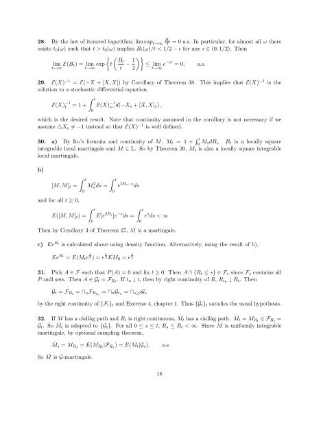
28. By the law of iterated logarithm, lim sup t t→∞ t
= 0 a.s. In particular, for almost all ω there
exists t 0 (ω) such that t > t 0 (ω) implies B t (ω)/t < 1/2 − ɛ for any ɛ ∈ (0, 1/2). Then
{ (
lim E(B Bt
t) = lim exp t
t→∞ t→∞ t − 1 )}
≤ lim e −ɛt = 0, a.s.
2 t→∞
29. E(X) −1 = E(−X + [X, X]) by Corollary of Theorem 38. This implies that E(X) −1 is the
solution to a stochastic differential equation,
E(X) −1
t = 1 +
∫ t
0
E(X) −1
s− d(−X s + [X, X] s ),
which is the desired result. Note that continuity assumed in the corollary is not necessary if we
assume △X s ≠ −1 instead so that E(X) −1 is well defined.
30. a) By Ito’s formula and continuity of M, M t = 1 + ∫ t
0 M sdB s . B t is a locally square
integrable local martingale and M ∈ L. So by Theorem 20, M t is also a locally square integrable
local martingale.
b)
[M, M] t =
and for all t ≥ 0,
∫ t
0
E([M, M] t ) =
M 2 s ds =
∫ t
0
∫ t
0
e 2B s−s ds
E[e 2B s
]e −s ds =
∫ t
0
e s ds < ∞
Then by Corollary 3 of Theorem 27, M is a martingale.
c) Ee Bt is calculated above using density function. Alternatively, using the result of b),
Ee Bt = E(M t e t 2 ) = e
t
2 EM0 = e t 2
31. Pick A ∈ F such that P (A) = 0 and fix t ≥ 0. Then A ∩ {R t ≤ s} ∈ F s since F s contains all
P -null sets. Then A ∈ G t = F Rt . If t n ↓ t, then by right continuity of R, R tn ↓ R t . Then
G t = F Rt = ∩ n F Rt n
= ∩ nG tn = ∩ s≥t G s
by the right continuity of {F t } t and Exercise 4, chapter 1. Thus {G t } t satisfies the usual hypothesis.
32. If M has a càdlàg path and R t is right continuous, ¯Mt has a càdlàg path. ¯Mt = M Rt ∈ F Rt =
G t . So ¯M t is adapted to {G t }. For all 0 ≤ s ≤ t, R s ≤ R t < ∞. Since M is uniformly integrable
martingale, by optional sampling theorem,
¯M s = M Rs = E(M Rt |F Rs ) = E( ¯M t |G s ),
a.s.
So ¯M is G-martingale.
18