Solution to selected problems.

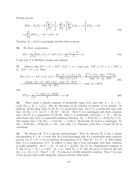
Poisson process,
⎡
C∑
t−s
E[N t − N s |F s ] = E ⎣
=µ
i=1
U i
⎤
⎦ =
∞∑
kP (C t−s = k) = µλ(t − s)
k=1
⎡
⎤
C ∞∑ ∑ t−s
E ⎣ U i |C t−s = k⎦ P (C t−s = k)
k=1
Therefore N t − µλt is a martingale and the claim is shown.
i=1
(53)
16. By direct computation,
1
1 − e −λh
λ(t) = lim P (t ≤ T < t + h|T ≥ t) = lim
h→0 h h→0 h
A case that T is Weibull is similar and omitted.
= λ. (54)
17. Observe that P (U > s) = P (T > 0, U > s) = exp{−µs}. P (T ≤ t, U > s) = P (U >
s) − P (T > t.U > s). Then
∫ t+h
P (t ≤ T < t + h, t ≤ U) t
e −µt (λ + θt)e −(λ+θt)u du
P (t ≤ T < t + h|T ≥ t, U ≥ t) = =
P (t ≤ T, t ≤ U)
exp{−λt − µt − θt 2 }
and
= −1[exp{−λ(t + h) − θt(t + h)} − exp{−λt − θt2 }]
exp{−λt − θt 2 }
= 1 − exp{−(λ + θt)h}
λ # 1 − exp{−(λ + θt)h}
(t) = lim
= λ + θt (56)
h→0 h
18. There exists a disjoint sequence of predictable times {T n } such that A = {t > 0 :
△〈M, M〉 t ≠ 0} ⊂ ∪ n [T n ]. (See the discussion in the solution of exercise 12 for details.) In
addition, all the jump times of 〈M, M〉· is a predictable time. Let T be a predictable time such
that 〈M, M〉 T ≠ 0. Let N = [M, M] − 〈M, M〉. Then N is a martingale with finite variation
since 〈M, M〉 is a compensator of [M, M]. Since T is predictable, E[N T |F T − ] = N T − . On the
other hand, since {F t } is a quasi-left-continuous filtration, N T − = E[N T |F T − ] = E[N T |F T ] = N T .
This implies that △〈M, M〉 T = △[M, M] T = (△M T ) 2 . Recall that M itself is a martingale. So
M T = E[M T |F T ] = E[M T |F T − ] = M T − and △M T = 0. Therefore △〈M, M〉 T = 0 and 〈M, M〉 is
continuous.
19. By theorem 36, X is a special semimartingale. Then by theorem 34, it has a unique
decomposition X = M + A such that M is local martingale and A is a predictable finite variation
process. Let X = N + C be an arbitrary decomposition of X. Then M − N = C − A. This implies
that A is a compensator of C. It suffices to show that a local martingale with finite variation
is locally integrable. Set Y = M − N and Z = ∫ t
0 |dY s|. Let S n be a fundamental sequence of
Y and set T n = S n ∧ n ∧ inf{t : Z t > n}. Then Y Tn ∈ L 1 (See the proof of theorem 38) and
Z Tn ≤ n + |Y Tn | ∈ L 1 . Thus Y = M − N is has has a locally integrable variation. Then C is a sum
of two process with locally integrable variation and the claim holds.
22
(55)