TUTORIAL 5 SOLUTIONS #8.10.47 The Pareto distribution has ...
TUTORIAL 5 SOLUTIONS #8.10.47 The Pareto distribution has ...
TUTORIAL 5 SOLUTIONS #8.10.47 The Pareto distribution has ...

Create successful ePaper yourself
Turn your PDF publications into a flip-book with our unique Google optimized e-Paper software.
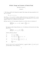
<strong>TUTORIAL</strong> 5 <strong>SOLUTIONS</strong><br />
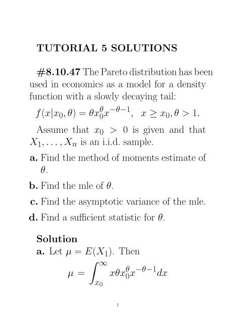
<strong>#8.10.47</strong> <strong>The</strong> <strong>Pareto</strong> <strong>distribution</strong> <strong>has</strong> been<br />
used in economics as a model for a density<br />
function with a slowly decaying tail:<br />
f(x|x 0 ,θ)=θx θ 0 x−θ−1 , x ≥ x 0 ,θ >1.<br />
Assume that x 0 > 0 is given and that<br />
X 1 ,...,X n is an i.i.d. sample.<br />
a. Find the method of moments estimate of<br />
θ.<br />
b. Find the mle of θ.<br />
c. Find the asymptotic variance of the mle.<br />
d. Find a sufficient statistic for θ.<br />
Solution<br />
a. Let µ = E(X 1 ). <strong>The</strong>n<br />
µ =<br />
∫ ∞<br />
x 0<br />
xθx θ 0 x−θ−1 dx<br />
1
= θx θ 0 ( x−θ+1<br />
−θ +1 )|∞ x 0<br />
= x 0θ<br />
θ − 1 .<br />
Thus θ = µ/(µ − x 0 ) and the method of<br />
moments estimate of θ is<br />
ˆθ =ˆµ 1 /(ˆµ 1 − x 0 )= ¯X/( ¯X − x 0 ).<br />
b. <strong>The</strong> loglikelihood function is<br />
n∏<br />
l(θ) = log[ θx θ 0 x−θ−1 i<br />
]<br />
Thus<br />
i=1<br />
= n log(θ)+nθ log(x 0 )<br />
n∑<br />
−(θ +1) log(x i ), x ≥ x 0 .<br />
i=1<br />
l ′ (θ) = n θ + n log(x 0) −<br />
n∑<br />
log(x i ).<br />
i=1<br />
2
Solving for l ′ (θ) = 0, the mle of θ is given<br />
by<br />
n<br />
˜θ = ∑ ni=1<br />
log(X i ) − n log(x 0 ) .<br />
c. <strong>The</strong> asymptotic variance of the mle is<br />
1/[nI(θ)]. Now<br />
I(θ) =−E[ ∂2<br />
∂θ 2 log f(X 1|θ)]<br />
= −E{ ∂2<br />
∂θ 2[log(θ)<br />
+θ log(x 0 ) − (θ + 1) log(X 1 )]}<br />
= 1 θ 2.<br />
Hence the asymptotic variance of the mle ˜θ<br />
is θ 2 /n.<br />
3
d. Observe that the joint pdf of X =<br />
(X 1 ,...,X n )is<br />
n∏<br />
f(x|θ) =<br />
where<br />
i=1<br />
θx θ 0 x−θ−1 i<br />
= θ n x nθ<br />
0 ( n ∏<br />
i=1<br />
= g(t, θ)h(x),<br />
t =<br />
n∏<br />
x i ,<br />
i=1<br />
x i ) −θ−1<br />
g(t, θ) =θ n x nθ<br />
0 t−θ−1 ,<br />
h(x) =1.<br />
By the factorization theorem, T (X) = ∏ n<br />
i=1 X i<br />
is sufficient for θ.<br />
4
#8.10.53 Let X 1 ,...,X n be i.i.d. uniform<br />
on [0,θ].<br />
a. Find the method of moments estimate of<br />
θ and its mean and variance.<br />
b. Find the mle of θ.<br />
c. Find the probability density of the mle,<br />
and calculate its mean and variance. Compare<br />
the variance, the bias, and the mean<br />
squared error to those of the method of<br />
moments estimate.<br />
d. Find a modification of the mle that renders<br />
it unbiased.<br />
Solution<br />
a. Let µ = E(X 1 ). <strong>The</strong>n<br />
and θ =2µ.<br />
µ = 1 θ<br />
∫ θ<br />
0<br />
xdx = θ 2 ,<br />
5
Thus the method of moments estimate of<br />
θ is<br />
ˆθ =2ˆµ 1 =2¯X.<br />
Also,<br />
E(ˆθ) =2E( ¯X) =2( θ 2 )=θ,<br />
Var(ˆθ) = Var(2 ¯X) = 4 n Var(X 1)= θ2<br />
3n ,<br />
since<br />
Var(X 1 )= 1 ∫ θ<br />
x 2 dx − (EX<br />
θ<br />
1 ) 2 = θ2<br />
12 .<br />
b. <strong>The</strong> likelihood function is<br />
n∏ 1<br />
lik(θ) =<br />
θ I{x i ≤ θ}<br />
i=1<br />
0<br />
= 1<br />
θ nI{max(x 1,...,x n ) ≤ θ}.<br />
<strong>The</strong> maximum of lik(θ) occurs at θ = max(x 1 ,<br />
...,x n ) and hence the mle of θ is<br />
˜θ = max(X 1 ,...,X n ).<br />
6
c. Observe that the cdf of ˜θ is given by<br />
F˜θ(x) =P (˜θ ≤ x)<br />
= P (max(X 1 ,...,X n ) ≤ x)<br />
n∏<br />
= P (X i ≤ x)<br />
i=1<br />
=( x θ )n .<br />
<strong>The</strong> pdf f˜θ(x) is<br />
f˜θ(x) = d<br />
dx F˜θ(x) = nxn−1<br />
θ n ,<br />
whenever 0 ≤ x ≤ θ. Also,<br />
E(˜θ) = 1 ∫ θ<br />
θ n nx n dx =<br />
nθ<br />
0 n +1 ,<br />
bias = E(˜θ) − θ = −<br />
θ<br />
n +1 ,<br />
Var( ˜θ) = 1 ∫ θ<br />
θ n nx n+1 dx − ( nθ<br />
n +1 )2<br />
=<br />
0<br />
nθ 2<br />
(n +1) 2 (n +2) .<br />
7
<strong>The</strong> MSE of ˜θ is<br />
MSE(˜θ) =Var(˜θ) + Bias 2<br />
=<br />
=<br />
nθ 2<br />
(n +1) 2 (n +2) +(− θ<br />
n +1 )2<br />
2θ 2<br />
(n + 1)(n +2) .<br />
Comparison of ˆθ and ˜θ<br />
Even though ˆθ is an unbiased estimator<br />
of θ while ˜θ is a biased estimator of θ, the<br />
MSE of ˜θ is dramatically smaller (for large<br />
n) than the MSE of ˆθ.<br />
d. <strong>The</strong> following modification of the mle<br />
makes it unbiased:<br />
θ ∗ (n +1)˜θ<br />
=<br />
n<br />
since<br />
E(θ ∗ )= n +1<br />
n<br />
E(˜θ) =θ.<br />
8
#8.10.57 This problem is concerned with<br />
the estimation of the variance of a normal<br />
<strong>distribution</strong> with unknown mean from a sample<br />
X 1 ,...,X n of i.i.d. normal random variables.<br />
In answering the following questions,<br />
use the fact that (from <strong>The</strong>orem B of Section<br />
6.3)<br />
(n − 1)s 2<br />
∼ χ 2 n−1<br />
σ 2<br />
and that the mean and variance of a chisquare<br />
random variable with r df are r and<br />
2r respectively.<br />
a. Which of the following estimates is unbiased?<br />
s 2 = 1 n∑<br />
(X<br />
n − 1 i − ¯X) 2 ,<br />
i=1<br />
ˆσ 2 = 1 n∑<br />
(X<br />
n i − ¯X) 2 .<br />
i=1<br />
9
. Which of the estimates given in part (a)<br />
<strong>has</strong> the smaller MSE?<br />
c. For what value of ρ does<br />
n∑<br />
ρ (X i − ¯X) 2<br />
i=1<br />
have the minimal MSE?<br />
Solution<br />
a. Recall from Section 6.3 that (n−1)s 2 /σ 2 ∼<br />
χ 2 n−1 <strong>distribution</strong>. Hence<br />
(n − 1)s2<br />
E<br />
σ 2 = n − 1<br />
which implies that<br />
E(s 2 )=σ 2 ,<br />
E(ˆσ 2 )= n − 1<br />
n σ2 .<br />
Thus s 2 is an unbiased estimate of σ 2 .<br />
10
. Since (n − 1)s 2 /σ 2 ∼ χ 2 n−1 <strong>distribution</strong>,<br />
we have<br />
(n − 1)s2<br />
Var(<br />
σ 2 )=2(n − 1).<br />
Thus<br />
Var(s 2 )=<br />
2σ4<br />
n − 1 ,<br />
Var(ˆσ 2 ) = Var( n − 1 2(n −<br />
n s2 1)σ4<br />
)=<br />
n 2 ,<br />
MSE(s 2 ) = Var(s 2 )+[E(s 2 ) − σ 2 ] 2<br />
= 2σ4<br />
n − 1 ,<br />
MSE(ˆσ 2 ) = Var(ˆσ 2 )+[E(ˆσ 2 ) − σ 2 ] 2<br />
=<br />
=<br />
2(n − 1)σ4<br />
n 2 + σ4<br />
n 2<br />
(2n − 1)σ4<br />
n 2 .<br />
11
Consequently we conclude that ˆσ 2 <strong>has</strong> the<br />
smaller MSE since<br />
c. Let<br />
MSE(ˆσ 2 ) < MSE(s 2 ).<br />
n<br />
ˆσ ρ 2 = ρ ∑<br />
(X i − ¯X) 2 .<br />
i=1<br />
<strong>The</strong>n ˆσ 2 ρ =(n − 1)ρs2 . As in part (b), we<br />
have<br />
E(ˆσ ρ)=(n 2 − 1)ρσ 2 ,<br />
Var(ˆσ ρ)=(n 2 − 1) 2 ρ 2 Var(s 2 )<br />
=2(n − 1)ρ 2 σ 4 .<br />
12
Finally,<br />
and<br />
MSE(ˆσ ρ)<br />
2<br />
=Var(ˆσ ρ)+[E(ˆσ 2 ρ) 2 − σ 2 ] 2<br />
=2(n − 1)ρ 2 σ 4 +[nρσ 2 − (ρ +1)σ 2 ] 2<br />
= σ 4 (1 + 2ρ − 2nρ − ρ 2 + n 2 ρ 2 ).<br />
d<br />
dρ MSE(ˆσ2 ρ )<br />
= σ 4 (2 − 2n − 2ρ +2n 2 ρ).<br />
Solving for (d/dρ)MSE(ˆσ ρ 2 ) = 0, we obtain<br />
ρ = 1<br />
n +1 .<br />
ˆσ ρ 2 <strong>has</strong> the smallest MSE when ρ =1/(n +<br />
1).<br />
13
#8.10.60 Let X 1 ,...,X n be an i.i.d. sample<br />
from an exponential <strong>distribution</strong> with<br />
the density function<br />
f(x|τ) = 1 τ e−x/τ , 0 ≤ x
g. Find the form of an exact confidence interval<br />
for τ.<br />
Solution<br />
a. Writing X =(X 1 ,...,X n ), the loglikelihood<br />
function is<br />
n∏ 1<br />
l(τ) = log<br />
τ e−x i/τ<br />
Also,<br />
i=1<br />
= −n log(τ) − 1 τ<br />
l ′ (τ) =− n τ + 1<br />
τ 2<br />
n ∑<br />
i=1<br />
n∑<br />
x i .<br />
i=1<br />
x i .<br />
Solving for l ′ (τ) = 0, the mle of τ is<br />
ˆτ = ¯X.<br />
15
. We note from Chapter 4.5 of the text<br />
that<br />
S = X 1 + ···+ X n ∼ Γ(n, 1 τ ).<br />
Hence the pdf of ¯X = S/n is<br />
f ¯X(x) =<br />
sn−1<br />
τ n Γ(n) e−s/τ | ds<br />
dx |<br />
= nn x n−1<br />
τ n Γ(n) e−nx/τ , x > 0,<br />
which is the pdf of the Γ(n, n/τ) <strong>distribution</strong>.<br />
c. and d. Since ¯X ∼ Γ(n, n/τ), we have<br />
E( ¯X) =τ,<br />
Var( ¯X) = τ 2<br />
n .<br />
From the CLT, ( ¯X − τ)/ √ τ 2 /n is approximately<br />
distributed as N(0, 1) for large n.<br />
16
e. <strong>The</strong> Cramér-Rao lower bound is 1/[nI(τ)]<br />
where<br />
I(τ) =−E[ ∂2<br />
∂τ 2 log(1 τ e−X1/τ )]<br />
= − 1<br />
τ 2 + E(2X 1<br />
τ 3 )<br />
= 1<br />
τ 2,<br />
since E(X 1 ) = τ. This implies that the<br />
Cramér-Rao lower bound is<br />
[nI(τ)] −1 = τ 2 /n.<br />
This lower bound equals the variance of ¯X.<br />
Hence we conclude that there is no other<br />
unbiased estimate of τ with a smaller variance<br />
than ¯X.<br />
17
f. From part (c), we have ( ¯X −τ)/ √ τ 2 /n<br />
is approximately distributed as N(0, 1) for<br />
large n.<br />
Hence an approximate 100(1 − α)% CI for<br />
τ is<br />
¯X ± z 1−α/2<br />
τ<br />
√ n<br />
≈ ¯X ± z 1−α/2<br />
¯X√n ,<br />
or equivalently the set of τ’s satisfying<br />
τ<br />
τ − z 1−α/2 √ ≤ ¯X τ<br />
≤ τ + z n 1−α/2 √ . n<br />
18
g. Note that ¯X <strong>has</strong> exactly the Γ(n, n/τ)<br />
<strong>distribution</strong>.<br />
Let G τ (α) denote the 100α percentile of<br />
the Γ(n, n/τ) <strong>distribution</strong>, i.e.<br />
P ( ¯X ≤ G τ (α)) = α.<br />
<strong>The</strong>n an exact 100(1 − α)% CI for τ is<br />
given by the set of τ’s satisfying<br />
G τ (α/2) ≤ ¯X ≤ G τ (1 − α/2).<br />
19