4 Comparison of the ALMA and Herschel - ESO

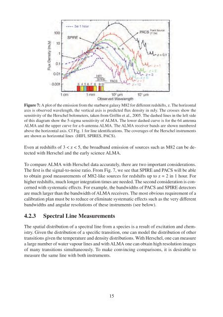
Figure 7: A plot of the emission from the starburst galaxy M82 for different redshifts, z. The horizontal
axis is observed wavelength, the vertical axis is predicted flux density in mJy. The crosses show the
sensitivity of the Herschel bolometers, taken from Griffin et al., 2005. The dashed lines in the left side
of this diagram show the 5-sigma sensitivity of ALMA. The lower dashed curve is for the 64 antenna
ALMA and the upper curve for a 6-antenna ALMA. The ALMA receiver bands are shown numbered
above the horizontal axis. Cf Fig. 1 for line identifications. The coverages of the Herschel instruments
are shown as horizontal lines (HIFI, SPIRES, PACS).
Even at redshifts of 3 < z < 5, the broadband emission of sources such as M82 can be detected
with Herschel and the early science ALMA.
To compare ALMA with Herschel data accurately, there are two important considerations.
The first is the signal-to-noise ratio. From Fig. 7, we see that SPIRE and PACS will be able
to obtain good measurements of M82-like sources for redshifts up to z = 2 in 1 hour. For
higher redshifts, much longer integration times are needed. The second consideration is concerned
with systematic effects. For example, the bandwidths of PACS and SPIRE detectors
are much larger than the bandwidth of ALMA receivers. The most obvious requirement of a
calibration plan must be to reduce or eliminate systematic effects such as the very different
bandwidths and angular resolutions of these instruments (see below).
4.2.3 Spectral Line Measurements
The spatial distribution of a spectral line from a species is a result of excitation and chemistry.
Given the distribution of a specific transition, one can model the distribution of other
transitions given the temperature and density distributions. With Herschel, one can measure
a large number of water vapour lines and with ALMA one can obtain high resolution images
of many transitions simultaneously. To make convincing comparisons, it is desirable to
measure the same line with both instruments.
15