Remote sensing of natural hazards
Remote sensing of natural hazards
Remote sensing of natural hazards

You also want an ePaper? Increase the reach of your titles
YUMPU automatically turns print PDFs into web optimized ePapers that Google loves.
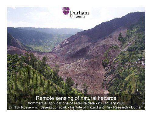
<strong>Remote</strong> <strong>sensing</strong> <strong>of</strong> <strong>natural</strong> <strong>hazards</strong><br />
Commercial applications <strong>of</strong> satellite data - 28 January 2009<br />
Dr Nick Rosser– n.j.rosser@dur.ac.uk - Institute <strong>of</strong> Hazard and Risk Research - Durham<br />
University
<strong>Remote</strong> Sensing & Natural Hazards<br />
Research<br />
• Introduction to IHRR<br />
– Combine social & physical approaches to<br />
understanding hazard & risk<br />
– ‘Global South’ focus<br />
– Applied & responsive research<br />
– Flooding, EQs & Landslides<br />
• IHRR application <strong>of</strong> RS to NH research<br />
• Process understanding &modelling<br />
• Linking process to earth observation<br />
• Prediction &upscaling<br />
– Coastal change<br />
– Post-earthquake sedimentation<br />
www.dur.ac.uk/ihrr<br />
• Future research directions &<br />
challenges<br />
Hazards research v <strong>hazards</strong> impact
Monitoring processes<br />
Rock cliff retreat – influence <strong>of</strong> precision<br />
• Challenges . . .<br />
– Input data for coastline retreat prediction<br />
– Poor quality monitoring data, looking in the<br />
wrong direction?<br />
– Resolution & sampling frequency<br />
• Integrating air-borne with terrestrial remote<br />
<strong>sensing</strong> data to better interpret remote<br />
<strong>sensing</strong> data<br />
• 3D laser scanning survey at 0.01 m<br />
resolution, over > 50,000 m 2 <strong>of</strong> cliff face<br />
• 3D modelling <strong>of</strong> scan data can detect 3D<br />
change to the cliff face < 0.0001 m 3
3D data processing &rockfall geometry extraction<br />
NJ Rosser, DN Petley, M. Lim, SA Dunning & RJ Allison 2005 Terrestrial laser scanning for monitoring the process <strong>of</strong><br />
hard rock coastal cliff erosion Quarterly Journal <strong>of</strong> Engineering Geology and Hydrogeology, 38, 363–375
Reassessing retreat<br />
654,373 rockfalls monitored over 5 years (mean = 0.001 m 3 , largest = 2,500 m 3 )<br />
Aggregate recession rate = 0.01 m/yr (published rate = 0.1 m/yr)<br />
Predicted 100 yr retreat = 3.6 m (published prediction 100 yr retreat – 90 m)
Sea-level control on cliff erosion rate?<br />
3D data processing &rockfall geometry extraction<br />
NJ Rosser, DN Petley, M. Lim, SA Dunning & RJ Allison 2005 Terrestrial laser scanning for monitoring the process <strong>of</strong><br />
hard rock coastal cliff erosion Quarterly Journal <strong>of</strong> Engineering Geology and Hydrogeology, 38, 363–375
Environmental control on rockfall occurrence?<br />
3D data processing &rockfall geometry extraction<br />
NJ Rosser, DN Petley, M. Lim, SA Dunning & RJ Allison 2005 Terrestrial laser scanning for monitoring the process <strong>of</strong><br />
hard rock coastal cliff erosion Quarterly Journal <strong>of</strong> Engineering Geology and Hydrogeology, 38, 363–375<br />
Squares represent 11 m x 11 m <strong>of</strong> cliff face, at monthly<br />
survey intervals
Precursors & failure prediction?<br />
•3D assessment identifies precursors<br />
•Potential to predict v forecast<br />
•Applied more widely to:<br />
•Embankments<br />
•Mine high-walls<br />
•Permanent monitoring<br />
3D data processing &rockfall geometry extraction<br />
Rosser, N.J., Lim, N, Petley, D.N., Dunning, S. & Allison, R.J. 2007 Patterns <strong>of</strong> precursory rockfall prior to slope failure.<br />
Journal <strong>of</strong> Geophysical Research.<br />
Squares represent 11 m x 11 m <strong>of</strong> cliff face, at monthly<br />
survey intervals
Post-earthquake<br />
landslides &<br />
sedimentation<br />
•EQ triggered landslide<br />
potentially hold great insight<br />
into earthquake dynamics &<br />
prediction<br />
•History <strong>of</strong> extreme postearthquake<br />
landscape change<br />
& sedimentation<br />
Sichuan<br />
2008<br />
(after, Bilham (2007))<br />
•What is the likely future nature<br />
<strong>of</strong> sediment dynamics in post-<br />
EQ Sichuan?<br />
Challenges:<br />
•Limited image availability<br />
•Topography<br />
•Monsoon<br />
•Politically sensitive<br />
(after, Keefer (1990))
Post 1999 Chi Chi, Taiwan river-bed<br />
aggradation<br />
1998<br />
2005<br />
2004
Post-earthquake<br />
sedimentation –<br />
Sichuan?<br />
17 June<br />
18 Nov<br />
Aggradation <strong>of</strong> >10 m in Beichuan in 5<br />
months, due to landslide remobilization
Steep topography - Poor lighting - Monsoon conditions - Data access<br />
http://www.eeri.org/site/images/lfe/china_20080512_zwang.ppt
http://www.eeri.org/site/images/lfe/china_20080512_zwang.ppt<br />
Continuing collapse – Monsoon driven failure<br />
http://www.eeri.org/site/images/lfe/china_20080512_zwang.ppt
Combined use <strong>of</strong> ALOS, EO1, QB, & SPOT imagery
Post-EQ<br />
sedimentation<br />
Automatic landslide mapping<br />
Combined multispectral analysis, using a<br />
range <strong>of</strong> available satellite imagery:<br />
•SPOT, IKONOS, LANDSAT, ALOS,<br />
EO1<br />
•Develop combine topographic / spectral<br />
model to classify landslides<br />
•Repeat over successive images<br />
Model <strong>of</strong> landslide distribution based<br />
upon:<br />
•Topographic amplification (DEM)<br />
•Slope / curvature<br />
•Ground cover (SPOT)<br />
Future EQ landslide prediction
30 % ground surface failed, > 100,000 landslides mapped, to date > 40,000<br />
reactivated
Post-EQ sedimentation<br />
Automatic landslide mapping<br />
•Modelled landslide<br />
distribution<br />
•Demonstrates limits<br />
to image resolution<br />
•Model transfer to<br />
other examples
Future research directions<br />
• Combining ground-based<br />
observations with wide-scale air<br />
&space-bourne monitoring<br />
• TLS, GB-InSAR<br />
• Potential for rapid assessment<br />
• Move towards predictive<br />
monitoring:<br />
• PSInSAR, TRMM, TLS<br />
• Temporal & spatial resolution<br />
• ? = ???????
www.dur.ac.uk/ihrr<br />
<strong>Remote</strong> <strong>sensing</strong> <strong>of</strong> <strong>natural</strong> <strong>hazards</strong><br />
Commercial applications <strong>of</strong> satellite data - 28 January 2009<br />
Dr Nick Rosser – n.j.rosser@dur.ac.uk - Institute <strong>of</strong> Hazard and Risk Research - Durham University
Flood modelling<br />
Why do we need satellite<br />
imagery for flood<br />
inundation modelling?<br />
1. Source <strong>of</strong> boundary<br />
condition data<br />
•Topography, especially<br />
given finer resolution models<br />
where topographic data<br />
handling is spatially explicit<br />
(e.g. 1.0 m resolution)<br />
•Friction, especially as it is<br />
controlled by land-use<br />
cover, although both<br />
theoretical arguments and<br />
sensitivity analysis points to<br />
inundation being less<br />
sensitive to floodplain<br />
friction but very sensitive to<br />
in-channel friction)<br />
York floods, 2000
2. In model parameterisation . . .<br />
• All flood inundation<br />
models are simplifications<br />
<strong>of</strong> the governing<br />
processes<br />
• Results in parameters<br />
with uncertain physical<br />
meaning (e.g. roughness)<br />
as they are effective<br />
• Need predictions that can<br />
be used to constrain<br />
those parameters<br />
• Inundation extent is really<br />
useful here<br />
York floods, 2000<br />
Yu, D. & Lane, S. 2005. Urban flood modelling using a 2-dimensional diffusionwave<br />
treatment. Hydrological Processes
3. For model validation<br />
100<br />
90<br />
Subject to data not being used in<br />
parameterisation, as a means <strong>of</strong><br />
assessing model performance<br />
Important when assessing<br />
different models<br />
Model performance<br />
80<br />
70<br />
60<br />
50<br />
40<br />
30<br />
Accuracy<br />
Conditional Kappa<br />
(for wet cells)<br />
4<br />
8<br />
16<br />
32<br />
32 m<br />
16 m<br />
8 m<br />
4 m