Microtremor Measurements Used to Map Thickness of Soft Sediments
Microtremor Measurements Used to Map Thickness of Soft Sediments
Microtremor Measurements Used to Map Thickness of Soft Sediments

You also want an ePaper? Increase the reach of your titles
YUMPU automatically turns print PDFs into web optimized ePapers that Google loves.
256 M. Ibs-von Seht and J. Wohlenberg<br />
Table 2<br />
Geotechnical Parameters <strong>Used</strong> <strong>to</strong> Calculate Transfer Functions<br />
for Sites M25, W21, W43, W41, $9, and E6<br />
Depth v s p<br />
Site Lithology (m) (lrdsec) (kg/m 3) Q<br />
M25 clay 0-10 303 2053 6.1<br />
sand 10-25 398 2090 8.5<br />
sand 25-44 465 2101 10.4<br />
hard rock >44 2500 2500 100<br />
W21 loess 0-8 200 1900 3.5<br />
gravel 8-14 300 2080 6<br />
sand 14-25 398 2090 8.5<br />
sand 25-50 482 2104 10.9<br />
sand 50-75 540 2112 12.6<br />
sand 75-100 585 2117 14<br />
sand 100-111 622 2120 15.2<br />
hard rock > 111 2500 2500 100<br />
W43 loess 0-8 200 1900 3.5<br />
gravel 8-15 300 2080 6<br />
sand 15-25 398 2090 8.5<br />
sand 25-50 482 2104 10.9<br />
sand 50-61 540 2107 12.6<br />
hard rock > 110 2500 2500 100<br />
W41 loess 0-8 200 1900 3.5<br />
gravel 8-14 300 2080 6<br />
sand 14-25 398 2090 8.5<br />
sand 25-50 482 2104 10.9<br />
sand 50-75 540 2112 12.6<br />
sand 75-100 585 2117 14<br />
sand 100-129 622 2120 15.2<br />
clay 129-140 475 2298 16.2<br />
hard rock >140 2500 2500 100<br />
$9 sand 0-25 398 2090 8.5<br />
sand 25-33 430 2095 9.4<br />
brown coal 33-35 216 1200 3<br />
sand 35-55 495 2104 11.3<br />
hard rock >55 2500 2500 100<br />
E6 gravel 0-15 353 1800 6<br />
gravel 15-25 410 1950 8<br />
gravel 25-35 452 2050 10<br />
sand 35-50 482 2102 10.9<br />
sand 50-100 585 2113 14<br />
sand 100-150 654 2118 16.2<br />
sand 150-200 709 2122 18<br />
sand 200-250 754 2124 19.5<br />
sand 250-300 793 2125 20.9<br />
sand 300-350 828 2127 22<br />
sand 350-400 859 2127 23.1<br />
sand 400-450 888 2128 24.1<br />
sand 450-485 907 2129 24.8<br />
sand 485-520 600 3000 25.4<br />
sand 520-565 946 2129 26.2<br />
hard rock >565 3100 2800 120<br />
The deviations <strong>of</strong> the data points in Figure 7 from the<br />
strict linear relationships are most probably a consequence<br />
<strong>of</strong> lithological inhomogeneties. Equations (10) and (11) are<br />
based on the assumption <strong>of</strong> equal v~(z) functions at each site<br />
measured. Conditions in practice are different because there<br />
may occur layers <strong>of</strong> velocities more or less deviating from<br />
a general velocity-depth function. Thus, drawing a straight<br />
line through the data points includes an averaging <strong>of</strong> lithol-<br />
E<br />
¢/)<br />
u)<br />
¢.-<br />
1000"<br />
o 100"<br />
. i<br />
t'-<br />
E<br />
E<br />
°~<br />
(D<br />
10-<br />
0.1<br />
% i i i i i I i i J i t<br />
,~, ', resonant frequencies : ',<br />
~,,~, calculated, , , on, the, base eq., (5) ,i ::<br />
L<br />
i % i i i i ~ I i ___L._ _L------I...<br />
["........ ~-X~';T---r'-r'~-,-rn-~ ..... , - , , ;<br />
[__ K _-_--:i: -_-~'i._,_ _~_ zero weighted data points.<br />
l ; :\~ ...... J .L . ,<br />
. . . . . . . . . . . . . v . . . . . T-v-t-1 . . . . . . r . . . . r---t---<br />
[ ...... ; .... ,*-"~.: ~x . . . . F ,"h", , , ,<br />
i i q ",1 i i i i t • i ~ i<br />
f ........ ~ .... ~---~:-x,-,-~,4-,, . . . . . ~-~ .... ,---~--<br />
/<br />
i<br />
',<br />
i<br />
',<br />
i<br />
',<br />
'.1 i i i<br />
~:.4_\, ,/,<br />
~l<br />
,,<br />
i<br />
,<br />
i<br />
,<br />
i<br />
I" ........ . . L ..... . ! -- - L- -II I .~,l~lt. f%~. -~., ~_ J- ~ J~ ..... ~L4 .... -t ---L--I I<br />
= mare Trequenoes4/,iK;... ,'NL 2~x a" '\ ' '<br />
,n N-s dra "4 i<br />
l<br />
........ k .... *-----~----~-- ~--4 ~~ Z. " --..%~ .... ~---~---<br />
........ L .... S---.L----t..~--~.U J . . . . t: ---_l~--t.---<br />
t . . . . . . . . ~ - J ' " . . . .<br />
£ . T------F----r--~--T--FS-- -¥--~ . . . . . . . . . . . -r-%- --<br />
F ........ ,, ,,,<br />
i i . , *~ i t<br />
............. ~-ma n frequendes-~ .... ,--,-,~<br />
: , • , "... , ,,: ,<br />
I- ........ ~ .... ,- in S/R-speetra---~'~.,.;--~.~ -<br />
........ ,~ .... I---,~-",-- ; -'-~'" ," '--~'U -<br />
t I t I I t l t . . . .<br />
1 5<br />
frequency [Hz]<br />
Figure 7. Main frequencies in spectral ratios plotted<br />
versus sediment thickness (solid circles: H/V frequencies;<br />
triangles: S/R frequencies). The solid lines<br />
are fits <strong>to</strong> the data points (see equation 9). The dashed<br />
line is the theoretical dependence between thickness<br />
and resonant frequency (see equation 5).<br />
Table 3<br />
Squared Correlation Coefficient (Rs) <strong>of</strong> Data Points in Figure 7<br />
and Values <strong>of</strong> a and b in Equation (9) with Standard Errors<br />
(Aa and Ab)<br />
S/RSpec~a<br />
H/VSpec~a<br />
R s 0.749 0.981<br />
a 146 96<br />
Aa 19 4<br />
b - 1.375 - 1.388<br />
Ab 0.210 0.025<br />
ogy or an averaging <strong>of</strong> the depth dependence <strong>of</strong> the shearwave<br />
velocity. A thickness value calculated from (10) or<br />
(11) for a particular site can only be as reliable as the overall<br />
vs(z) function is valid for the site. The very local subsurface<br />
velocity structure cannot be taken in<strong>to</strong> account for the calculation.<br />
However, especially for the H/V frequencies, the<br />
thickness-frequency correlation delivers an estimate <strong>of</strong> the<br />
local thickness that can be used for hard-rock basement mappings.<br />
A reason for the numerous outliers <strong>of</strong> S/R frequencies<br />
in Figure 7 and the high scatter <strong>of</strong> the data points in Figure<br />
8 could be the value <strong>of</strong> the noise level at the recording sites.<br />
Therefore, in Figure 9, we plotted the frequency ratio f~s/R)/<br />
f~wv) versus the horizontal rms amplitudes <strong>of</strong> the noise recordings<br />
(the amplitudes <strong>of</strong> the two horizontal records were<br />
averaged). The cross-plot illustrates that the frequency ratio<br />
becomes unstable and generally tends <strong>to</strong> higher values at