Predicting and evaluating extreme weather events

Predicting and evaluating extreme weather events
12th Experimental Chaos and Complexity Conference
18 May 2012
Ann Arbor, Michigan
Eric Gilleland
E-mail: EricG @ ucar.edu
Research Applications Laboratory,
National Center for Atmospheric Research (NCAR)
Weather and Climate Impacts Assessment Science (WCIAS) Program
Photo by Everett Nychka

Motivation: Defining Extreme Events
Pr{Winning ≥ $10, 000 in one drawing} ≈
0.000001306024

Motivation: Defining Extreme Events
Pr{Winning ≥ $10, 000 in one drawing} ≈
0.000001306024
Hereafter, simplify the problem by ignoring the fact we can win small
amounts, etc.

Motivation
Colorado Lottery
Pr{Winning ≥ $10, 000 in one drawing} ≈
0.000001306024
In ten years, playing one ticket
everyday, Pr{Winning ≥ $10, 000} ≈
0.004793062

Motivation
Colorado Lottery
Pr{Winning ≥ $10, 000 in one drawing} ≈
0.000001306024
In ten years, playing one ticket
everyday, Pr{Winning ≥ $10, 000} ≈
0.004793062
In 100 years ≈ 0.05003321
In 1000 years ≈ 0.7686185

Motivation
Colorado Lottery
Pr{Winning ≥ $10, 000 in one drawing} ≈
0.000001306024
In 1000 years ≈ 0.7686185
In ten years, playing one ticket
everyday, Pr{Winning ≥ $10, 000} ≈
0.004793062
In 100 years ≈ 0.05003321
Law of small numbers: events with small probably rarely happen, but
have many opportunities to happen. These follow a
Poisson distribution.

Motivation
Colorado Lottery
Can also talk about waiting time probability. The exponential
distribution models this.

Motivation
Colorado Lottery
Can also talk about waiting time probability. The exponential
distribution models this. For example, the probability that it will
take longer than a year to win the lottery (at one ticket per day) is
≈ 0.999523, longer than ten years ≈ 0.9952411, longer than 500 years
≈ 0.7877987, and so on (decays exponentially, but with a very slow
rate).

Motivation
Colorado Lottery
Another way to put it is that the expected number of years that it
will take to win more than $10,000 in the lottery (buying one ticket
per day) is about 2,096 years. If a ticket costs $1, then we can expect
to spend $765,682.70 before winning at least $10,000.

Motivation
Law of Large Numbers, Sum Stability, Central Limit Theorem
And other results give theoretical support for use of the
Normal distribution for analyzing most data.

Background: Extreme Value Theory (EVT)
Extremal Types Theorem
Theoretical support for using the Extreme Value Distributions
(EVD’s) for extrema.
• Valid for maxima over very large blocks, or
• Excesses over a very high threshold.
It is possible that there is no valid distribution for extremes of a given
random variable, but if one exists, it must be from the Generalized
Extreme Value (GEV) family (block maxima) or the Generalized
Pareto (GP) family (excesses over a high threshold). The two families
are related.
Poisson process allows for a nice characterization of the threshold
excess model that neatly ties it back to the GEV distribution.

Background
GEV
Three parameters: location,
scale and shape.
Pr{M n ≤ z} =
{
exp − [ 1 + ξ ( )] }
z−µ −1/ξ
σ
M n = max{X 1 , . . . , X n }
Simulated Maxima from various df’s.

Background
GEV
Three parameters: location, scale and shape.
{ [ ( )] } −1/ξ z − µ
Pr{X ≤ z} = exp − 1 + ξ
σ
Three types of tail behavior:
1. Bounded upper tail (ξ < 0, Weibull), Temperature, Wind Speed,
Sea Level
2. light tail (ξ = 0, Gumbel), and
3. heavy tail (ξ > 0, Fréchet), Stream Flow, Precipitation, Economic
Impacts.
Analogous situation for threshold excess approach, but focus is on the
tail of these distributions.

Background
Block Maxima vs. POT

Background
Block Maxima vs. POT

Background
Block Maxima vs. POT

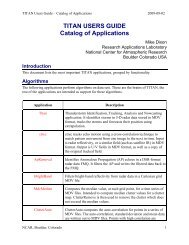
Example
Fort Collins, Colorado
daily precipitation amount
• Time series of daily precipitation
amount (inches), 1900–1999.
• Semi-arid region.
• Marked annual cycle in precipitation
(wettest in late spring/early summer,
driest in winter).
• No obvious long-term trend.
• Recent flood, 28 July 1997.
(substantial damage to
Colorado State University)
http://ccc.atmos.colostate.edu/~odie/rain.html

Examples
Fort Collins, Colorado precipitation
Gumbel hypothesis rejected at 5% level.
ξ ≈ 0.17, 95% CI ≈ (0.01, 0.37)
Fréchet (heavy tail)
10-year return level
≈ 2.8 in.
Pr{M n ≥ 3 in} ≈ 0.08
Return period for
3 in. is ≈ 12.5 years

Extremes vs Extreme Impacts
Extremes
May or may not have an extreme impact depending on various factors
(e.g., location, duration).
Combinations of ordinary conditions
Frozen ground and rain (e.g., 1959 Ohio statewide flood).

Weather Spells: Many ways to define them technically
Photo from NCAR’s
digital image library,
DIO1492
Do extremes of lengths of spells follow EV df’s? (e.g., Cebrián and
Abaurrea (2006), J. Hydrometeorology, 7, 713–723, use a marked
Poisson process approach)
The same type of weather spell may or may not be important
depending on where it occurs.

What is a drought?
"a period of abnormally dry weather sufficiently prolonged for the lack
of water to cause serious hydrologic imbalance in the affected area."
-Glossary of Meteorology (1959)
Meteorological–a measure of departure of precipitation from normal.
Due to climatic differences, what might be considered a drought
in one location of the country may not be a drought in another
location.
Agricultural–refers to a situation where the amount of moisture in
the soil no longer meets the needs of a particular crop.
Hydrological–occurs when surface and subsurface water supplies are
below normal.
Socioeconomic–refers to the situation that occurs when physical
water shortages begin to affect people.
http://www.wrh.noaa.gov/fgz/science/drought.php?wfo=fgz

Scale of Extreme Atmospheric Events
2006 European Heat Wave F5 Tornado in Elie Manitoba
(Fig. from KNMI) on Friday, June 22nd, 2007

Model/Reanalysis Resolution
Banff
●
Calgary
●
~40−km CFDDA reanalysis (1985−2005)
~200−km NCAR/NCEP reanalysis (1980−1999)
~150−km CCSM3 regional climate model

Severe Weather
As model resolution increases, some severe weather phenomena, such
as hurricanes, can be predicted. However, other types of severe weather
may still require higher resolution.
• Use large-scale indicators to analyze conditions ripe for severe
weather.
• Use climate models as drivers for finer scale weather models.
• Statistical approach to current trends in observations.
• Other?

Large-scale indicators for Severe weather
Non-severe
Severe
Significant
Non-tornadic
Significant
Tornadic
hail < 1.9 cm. (3/4 in.) diameter
winds < 55 kts. no tornado
Hail ≥ 1.9 cm. diameter
winds ≤ 55 kts. and < 65 kts. or tornado
Hail ≥ 5.07 cm. (2 in.) diameter
Winds ≥ 65 kts.
Same as sig. tornadic with F2 (or greater) tornado.

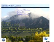
Large-scale indicators for Severe weather
CAPE×Shear WmSh=W max ×Shear (m 2 /s 2 )
0.00000 0.00010 0.00020
Non−severe
Severe
Significant Non−tornadic
Significant Tornadic
0.000 0.001 0.002 0.003
0.0 0.2 0.4 0.6 0.8 1.0
0.0 0.2 0.4 0.6 0.8 1.0
W max = √ 2 · CAPE
(m/s)
0e+00 2e+05 4e+05
0 2000 6000 10000

CAPE (W max ) and 0-6 km shear data, or indeed, output
Median AM cape*shear reanalysis (1980−1999)
25 30 35 40 45 50
200000
150000
100000
50000
0
−120 −110 −100 −90 −80 −70
NCAR/NCEP global reanalysis: 1.875 o × 1.915 o lon-lat grid, > 17K
points, 6-hourly, 1958–1999. See: Brooks et al. (2003), Atmos. Res.,
67–68, 73–94.

Large-scale indicators for Severe weather
WmSh=W max × Shear
AM Reanalysis (95-th quantile)
20-yr GEV return level
5000
4000
3000
2000
1000
0
Units are off here (shear is in knots instead of m/s, so take half of
what you see).

Large-scale indicators for Severe weather
GEV(µ(t) = µ 0 + µ 1 t, σ, ξ),
t = 0 (1958–1969), t = 1 (1970–1984), t = 2 (1985–1999).
20-year return levels (i.e., 95-th percentile, m/s).
1970−1984 vs 1958−1969
1985−1999 vs 1958−1969
1000
1000
500
500
0
0
−500
−500
Min. diff. from t = 0 to t = 2 is ≈ −750 m/s, max. is ≈ 400 m/s.
25th percentile of diff’s is ≈ −100 m/s, 75th percentile is ≈ 75 m/s.
−1000
−1000

Large-scale indicators for Severe weather
Threshold excess modeling using Bayesian Hierarchical Models (BHM)
Industrial Mathematical and Statistical Modeling (IMSM) Workshop
for Graduate Students. Center for Research in Scientific
Computation, Raleigh, North Carolina and the Statistical and
Applied Mathematical Sciences Institute (SAMSI), Research
Triangle Park, North Carolina, 20-28 July 2009.
Paper in Environmetrics, 22, 294–303:
Heaton, M.J., M. Katzfuss, S. Ramachandar, K. Pedings, Y.
Li, E. Gilleland, E. Mannshardt-Shamseldin, and R.L. Smith,
2009. Spatio-temporal models for extreme weather using largescale
indicators.

Large-scale indicators for Severe weather
Three models of increasing complexity applied to threshold excesses
(over the 95-th quantile of daily maximum WmSh).
Model 1: Very Simple
GPD with (ln) scale and shape parameter varying by region only.
y td (s l )|ψ u(sl )(s l ), ξ(s l ) iid ∼ GPD(ψ u(sl )(s l ), ξ(s l )), where
and
ln(ψ u(sl )(s l )) = α ψ + 1 sl ∈A ψ
δ ψ ,
ξ(s l ) = α ξ + 1 sl ∈A ξ
δ ξ ,
with A x somewhat arbitrarily chosen regions representing areas of
exceptional values of these parameters as estimated via MLE at
individual locations (this roughly translates to the “tornado alley").
Priors for these parameters are taken as α ψ ∼ N(5.5, 1), δ ψ ∼ N(0, 1),
α ξ ∼ N(0, 0.2 2 ), δ ξ ∼ N(0, 0.2 2 ).

Large-scale indicators for Severe weather
Model 2:
GPD with Gaussian process for the (ln) scale parameter, and shape
parameter varies according to region.
y td (s l )|ψ u(sl )(s l ), ξ(s l ) iid ∼ GPD(ψ u(sl )(s l ), ξ(s l )), where
ln(ψ u(sl )(s l )) ∼ GP ((µ ψ , τ 2 ψ, φ ψ ),
and
ξ(s l ) = α ξ + 1 sl ∈A ξ
δ ξ ,
with Cov(ln(ψ(s l )), ln(ψ(s k ))) = τ 2 exp{−φ ψ ‖s l − s k ‖}, and ‖ · ‖
the spherical distance in miles. Priors are the same as model 2, with
additional priors for µ ψ ∼ Unif(−∞, ∞), τψ 2 ∼ IG(2.1, 3), and
φ ψ ∼ Unif(0.001, 0.1).

Large-scale indicators for Severe weather
Model 3:
Point Process with temporal trend for location parameter, trivariate
Gaussian process for location and (ln) scale parameters, and shape
parameter varying according to region as in other two models.
x td (s l )|x td (s l ) > u(s l ), β 0 (s l ), β 1 (s l ), σ(s l ), ξ(s l ) iid ∼
where
and
PP(β 0 (s l ) + β 1 (s l )t, σ(s l ), ξ(s l )),
(β 0 (s l ), β 1 (s l ), ln(σ(s l ))) T ∼ GP 3 (µ M3 , φ M3 , Γ),
ξ(s l ) = α ξ + 1 sl ∈A ξ
δ ξ ,
with GP 3 a trivariate Gaussian process induced via coregionalization
(Gelfand et al. 2004), µ M3 = (µ β0 , µ β1 , µ σ ) T , φ M3 = (φ 1 , φ 2 , φ 3 ) T , and
Γ is a 3 × 3 lower triangular matrix with entries γ ij .

Large-scale indicators for Severe weather
Model 3 is best according to DIC (also most useful).
ˆβ 1 Values
Statistical Significance
1.0
Latitude
20 25 30 35 40 45
Latitude
4
20 25 30 35 40 45
2
0
−2
0.5
0.0
−0.5
−1.0
−120 −100 −80 −60
−120 −100 −80 −60
Longitude
Longitude
Is there practical significance with ˆβ 1 ranging only from about −4 to
4 (e.g., 4 × 42 years is only 168 m/s difference in location parameter)?

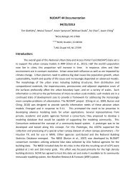
Large-scale indicators for Severe weather
Twenty-year return level differences as calculated from the posterior
means of Model 3 for 1999 vs 1958. Practical significance?
Latitude
20 25 30 35 40 45
60
40
20
0
−20
−120 −100 −80 −60
Longitude

Large-scale indicators for Severe weather
Conditional EVA
Heffernan and Tawn (2004), J. R. Statist. Soc. B, 66, 497–546.
• Allows as many variates as you like.
• Different assumptions than the usual multivariate EVA approach:
condition on one variable’s being large, and find the joint conditional
distribution of other variables.
• Uncertainty obtained through bootstrapping (can be slow).
• Model for positively associated pairs of r.v.’s has a simple form.
• Semi-parametric model.
• Theoretical justification for extrapolating beyond the range of the
sample.

Large-scale indicators for Severe weather
Conditional EVA
For simplicity, take the bivariate case, with random variables
X and Y .
1. Find marginal distributions, f X and f Y , using univariate EVT.
2. Transform X and Y to the Gumbel scale (w/o loss of generality).
3. Then, y|X = x = αx + x β Z, Z ∼ std. df., u a high threshold.
Ẑ =
y|X = x − ˆαx
.
Estimate α ∈ [0, 1] and β ∈ (−∞, 1) using, e.g., nls.
4. Using
x ˆβ
Ẑ, characterize f(Ẑ) (e.g., kernel density, resampling).
5. Sample at random from {Ẑi} n i=1 , calculate y (step 3), back-transform
(step 1).

Large-scale indicators for Severe weather
Conditional EVA
{ Y |X = x − αx
Pr
x β
}
≤ z|x > u
−→ G(z)
Joint tail behavior is characterized by α, β and G. G is not specified
by theory, and there is no assumption of multivariate regular variation.

Large-scale indicators for Severe weather
Mean Predicted WmSh (m/s) conditioned on high field energy
800
600
400
200
Performed using the texmex package in R

Summary/Conclusions/Discussion
• Defining extremes: Well-established statistical theory for events
with small probabilities of occurrence, but many chances to occur.
• Weather spells are trickier to analyze: dependent on location and
definition.
• Difficult to model severe weather events because of scale. Can use
large-scale indicators of environments conducive to having severe
weather.
• Analyzing extremes in the face of spatial dependence.
– Multivariate EVA, Copulas, BHM, EV df’s with spatial covariates.
Each is valid, and can be useful, but there are important
drawbacks to each.
– Conditional EVA (Heffernan and Tawn model) shows a lot of
promise. Still some drawbacks, but less important for most
studies.

http://www.assessment.ucar.edu/toolkit/
Software

Discussion
• How should extreme events be defined? Deadliness? Perceptionbased?
Statistically? Economically? Other?
• What is the relationship between changes in the mean and changes
in extremes? What about variability? Higher order moments?
• If climate models project the df of atmospheric variables, then do
they accurately portray the df’s? Enough so that functionals of
interest, such as extrema, are correctly characterized?
• If climate models only project the mean, then can anything be
said about extremes?
• How can it be determined if small changes in high values of largescale
indicators lead to a shift in the df of severe weather
conditional on the indicators?

Discussion
• How do we verify climate models, especially for inferring about
extremes?
• Extremes are often largely dependent on local conditions (e.g.,
topography, surface conditions, atmospheric phenomena, etc.), as
well as larger scale processes.
• Can a metric for climate change pertaining to extremes be
developed that makes sense, and provides reasonably accurate
information?
• How can uncertainty be characterized? Is there too much
uncertainty to make inferences about extremes?
• How can spatial structure be taken into account for extremes?
• Many extreme events, and especially extreme impact events, result
from multivariate processes. How can this be addressed?