Mining Frequent Itemsets – Apriori Algorithm

Laboratory Module 8
Mining Frequent Itemsets – Apriori Algorithm
Purpose:
− key concepts in mining frequent itemsets
− understand the Apriori algorithm
− run Apriori in Weka GUI and in programatic way
1 Theoretical aspects
In data mining, association rule learning is a popular and well researched method for discovering
interesting relations between variables in large databases. Piatetsky-Shapiro describes analyzing and
presenting strong rules discovered in databases using different measures of interestingness. Based on the
concept of strong rules, Agrawal introduced association rules for discovering regularities between products
in large scale transaction data recorded by point-of-sale (POS) systems in supermarkets. For example, the
rule {onion,potatoes}=>{burger} found in the sales data of a supermarket would indicate that if a customer
buys onions and potatoes together, he or she is likely to also buy burger. Such information can be used as
the basis for decisions about marketing activities such as, e.g., promotional pricing or product placements.
In addition to the above example from market basket analysis association rules are employed today in many
application areas including Web usage mining, intrusion detection and bioinformatics.
In computer science and data mining, Apriori is a classic algorithm for learning association rules.
Apriori is designed to operate on databases containing transactions (for example, collections of items
bought by customers, or details of a website frequentation). Other algorithms are designed for finding
association rules in data having no transactions (Winepi and Minepi), or having no timestamps (DNA
sequencing).
Definition:
Following the original definition by Agrawal the problem of association rule mining is defined as:
Let I = {i 1 , i 2 , ..., i n } be a set of n binary attributes called items. Let D = {t 1 , t 2 , ..., t n } be a set of
transactions called the database. Each transaction in D has a unique transaction ID and contains a subset of
the items in I. A rule is defined as an implication of the form X→Y where X, Y ⊆ I and ∩ = ∅. The
sets of items (for short itemsets) X and Y are called antecedent (left-hand-side or LHS) and consequent
(right-hand-side or RHS) of the rule respectively.
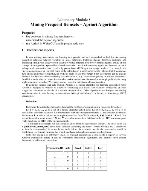
To illustrate the concepts, we use a small example from the supermarket domain. The set of items is I
= {milk,bread,butter,beer} and a small database containing the items (1 codes presence and 0 absence of
an item in a transaction) is shown in the table below. An example rule for the supermarket could be
{milk,bread}=>{butter} meaning that if milk and bread is bought, customers also buy butter.
Note: this example is extremely small. In practical applications, a rule needs a support of several
hundred transactions before it can be considered statistically significant, and datasets often contain
thousands or millions of transactions.
Transaction ID milk Bread butter beer
1 1 1 0 0
2 0 1 1 0
3 0 0 0 1
4 1 1 1 0
5 0 1 0 0

6 1 0 0 0
7 0 1 1 1
8 1 1 1 1
9 0 1 0 1
10 1 1 0 0
11 1 0 0 0
12 0 0 0 1
13 1 1 1 0
14 1 0 1 0
15 1 1 1 1
Useful Concepts
To select interesting rules from the set of all possible rules, constraints on various measures of
significance and interest can be used. The best-known constraints are minimum thresholds on support and
confidence.
Support
The support supp(X) of an itemset X is defined as the proportion of transactions in the data set which
contain the itemset.
supp(X)= no. of transactions which contain the itemset X / total no. of transactions
In the example database, the itemset {milk,bread,butter} has a support of 4 /15 = 0.26 since it occurs
in 26% of all transactions. To be even more explicit we can point out that 4 is the number of transactions
from the database which contain the itemset {milk,bread,butter} while 15 represents the total number of
transactions.
Confidence
The confidence of a rule is defined:
→ = ∪ /
For the rule {milk,bread}=>{butter} we have the following confidence:
supp({milk,bread,butter}) / supp({milk,bread}) = 0.26 / 0.4 = 0.65
This means that for 65% of the transactions containing milk and bread the rule is correct.
Confidence can be interpreted as an estimate of the probability P(Y | X), the probability of finding the RHS
of the rule in transactions under the condition that these transactions also contain the LHS.
Lift
The lift of a rule is defined as:
→ =
∪
∗
The rule {milk,bread}=>{butter} has the following lift:
supp({milk,bread,butter}) / supp({butter}) x supp({milk,bread})= 0.26/0.46 x 0.4= 1.4

Conviction
The conviction of a rule is defined as:
→ =
−
− →
The rule {milk,bread}=>{butter} has the following conviction:
1 – supp({butter})/ 1- conf({milk,bread}=>{butter}) = 1-0.46/1-0.65 = 1.54
The conviction of the rule X=>Y can be interpreted as the ratio of the expected frequency that X
occurs without Y (that is to say, the frequency that the rule makes an incorrect prediction) if X and Y were
independent divided by the observed frequency of incorrect predictions.
In this example, the conviction value of 1.54 shows that the rule {milk,bread}=>{butter} would be
incorrect 54% more often (1.54 times as often) if the association between X and Y was purely random
chance.
2. Apriori algorithm
General Process
Association rule generation is usually split up into two separate steps:
1. First, minimum support is applied to find all frequent itemsets in a database.
2. Second, these frequent itemsets and the minimum confidence constraint are used to form rules.
While the second step is straight forward, the first step needs more attention.
Finding all frequent itemsets in a database is difficult since it involves searching all possible itemsets
(item combinations). The set of possible itemsets is the power set over I and has size 2 n − 1 (excluding the
empty set which is not a valid itemset). Although the size of the powerset grows exponentially in the
number of items n in I, efficient search is possible using the downward-closure property of support (also
called anti-monotonicity) which guarantees that for a frequent itemset, all its subsets are also frequent and
thus for an infrequent itemset, all its supersets must also be infrequent. Exploiting this property, efficient
algorithms (e.g., Apriori and Eclat) can find all frequent itemsets.
Apriori Algorithm Pseudocode
procedure Apriori (T, minSupport) { //T is the database and minSupport is the minimum support
L1= {frequent items};
for (k= 2; L k-1 !=∅; k++) {
C k = candidates generated from L k-1
//that iscartesian product L k-1 x L k-1 and eliminating any k-1 size itemset that is not
//frequent
for each transaction t in database do{
#increment the count of all candidates in C k that are contained in t
L k = candidates in C k with minSupport
}//end for each
}//end for
return ⋃ ;
}
As is common in association rule mining, given a set of itemsets (for instance, sets of retail
transactions, each listing individual items purchased), the algorithm attempts to find subsets which are
common to at least a minimum number C of the itemsets. Apriori uses a "bottom up" approach, where
frequent subsets are extended one item at a time (a step known as candidate generation), and groups of
candidates are tested against the data. The algorithm terminates when no further successful extensions are
found.

Apriori uses breadth-first search and a tree structure to count candidate item sets efficiently. It
generates candidate item sets of length k from item sets of length k − 1. Then it prunes the candidates which
have an infrequent sub pattern. According to the downward closure lemma, the candidate set contains all
frequent k-length item sets. After that, it scans the transaction database to determine frequent item sets
among the candidates.
Apriori, while historically significant, suffers from a number of inefficiencies or trade-offs, which have
spawned other algorithms. Candidate generation generates large numbers of subsets (the algorithm attempts
to load up the candidate set with as many as possible before each scan). Bottom-up subset exploration
(essentially a breadth-first traversal of the subset lattice) finds any maximal subset S only after all 2 | S | − 1
of its proper subsets.
3. Sample usage of Apriori algorithm
A large supermarket tracks sales data by Stock-keeping unit (SKU) for each item, and thus is able to
know what items are typically purchased together. Apriori is a moderately efficient way to build a list of
frequent purchased item pairs from this data. Let the database of transactions consist of the sets {1,2,3,4},
{1,2,3,4,5}, {2,3,4}, {2,3,5}, {1,2,4}, {1,3,4}, {2,3,4,5}, {1,3,4,5}, {3,4,5}, {1,2,3,5}. Each number
corresponds to a product such as "butter" or "water". The first step of Apriori is to count up the frequencies,
called the supports, of each member item separately:
Item
1 6
2 7
3 9
4 8
5 6
Support
We can define a minimum support level to qualify as "frequent," which depends on the context.
For this case, let min support = 4. Therefore, all are frequent. The next step is to generate a list of all 2-pairs
of the frequent items. Had any of the above items not been frequent, they wouldn't have been included as a
possible member of possible 2-item pairs. In this way, Apriori prunes the tree of all possible sets. In next
step we again select only these items (now 2-pairs are items) which are frequent (the pairs written in bold
text):
Item Support
{1,2} 4
{1,3} 5
{1,4} 5
{1,5} 3
{2,3} 6
{2,4} 5
{2,5} 4
{3,4} 7
{3,5} 6
{4,5} 4

We generate the list of all 3-triples of the frequent items (by connecting frequent pair with frequent
single item).
Item
{1,3,4} 4
{2,3,4} 4
{2,3,5} 4
{3,4,5} 4
Support
The algorithm will end here because the pair {2,3,4,5} generated at the next step does not have the
desired support.
We will now apply the same algorithm on the same set of data considering that the min support is
5. We get the following results:
Step 1:
Step 2:
Item Support
1 6
2 7
3 9
4 8
5 6
Item Support
{1,2} 4
{1,3} 5
{1,4} 5
{1,5} 3
{2,3} 6
{2,4} 5
{2,5} 4
{3,4} 7
{3,5} 6
{4,5} 4
The algorithm ends here because none of the 3-triples generated at Step 3 have de desired support.

4. Sample usage of Apriori in Weka
For our test we shall consider 15 students that have attended lectures of the Algorithms and Data
Structures course. Each student has attended specific lectures. The ARFF file presented bellow contains
information regarding each student’s attendance.
@relation test_studenti
@attribute Arbori_binari_de_cautare {TRUE, FALSE}
@attribute Arbori_optimali {TRUE, FALSE}
@attribute Arbori_echilibrati_in_inaltime {TRUE, FALSE}
@attribute Arbori_Splay {TRUE, FALSE}
@attribute Arbori_rosu_negru {TRUE, FALSE}
@attribute Arbori_2_3 {TRUE, FALSE}
@attribute Arbori_B {TRUE, FALSE}
@attribute Arbori_TRIE {TRUE, FALSE}
@attribute Sortare_topologica {TRUE, FALSE}
@attribute Algoritmul_Dijkstra {TRUE, FALSE}
@data
TRUE,TRUE,TRUE,TRUE,FALSE,FALSE,TRUE,TRUE,FALSE,FALSE
TRUE,TRUE,TRUE,TRUE,TRUE,TRUE,FALSE,TRUE,FALSE,FALSE
FALSE,TRUE,TRUE,TRUE,FALSE,FALSE,FALSE,TRUE,FALSE,TRUE
FALSE,TRUE,FALSE,FALSE,TRUE,FALSE,TRUE,TRUE,FALSE,TRUE
TRUE,TRUE,FALSE,TRUE,TRUE,FALSE,TRUE,TRUE,FALSE,TRUE
TRUE,FALSE,TRUE,FALSE,FALSE,TRUE,TRUE,TRUE,FALSE,FALSE
FALSE,TRUE,FALSE,TRUE,TRUE,FALSE,TRUE,TRUE,FALSE,TRUE
TRUE,FALSE,TRUE,TRUE,TRUE,FALSE,TRUE,TRUE,TRUE,FALSE
FALSE,TRUE,TRUE,TRUE,TRUE,FALSE,FALSE,TRUE,FALSE,FALSE
TRUE,FALSE,TRUE,FALSE,TRUE,TRUE,FALSE,TRUE,FALSE,TRUE
FALSE,FALSE,TRUE,FALSE,TRUE,FALSE,FALSE,TRUE,TRUE,TRUE
TRUE,FALSE,FALSE,TRUE,TRUE,TRUE,FALSE,TRUE,FALSE,TRUE
FALSE,TRUE,TRUE,FALSE,TRUE,TRUE,FALSE,TRUE,FALSE,TRUE
TRUE,TRUE,TRUE,FALSE,FALSE,TRUE,FALSE,TRUE,FALSE,FALSE
TRUE,TRUE,FALSE,FALSE,TRUE,TRUE,FALSE,TRUE,FALSE,FALSE
Using the Apriori Algorithm we want to find the association rules that have minSupport=50%
and minimum confidence=50%. We will do this using WEKA GUI.
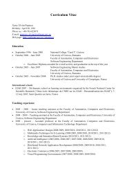
After we launch the WEKA application and open the TestStudenti.arff file, we move to the
Associate tab and we set up the following configuration:

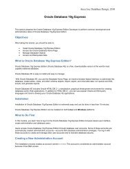
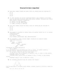
After the algorithm is finished, we get the following results:
If we look at the first rule we can see that the students who don’t attend the Sortare topologica
lecture have a tendency to attend the Arbori TRIE lecture. The confidence of this rule is 100% so it is very
believable. Using the same logic we can interpret all the the other rules that the algorithm has revealed.

The same results presented above can be obtained by implementing the WEKA Apriori Algorithm
in your own Java code. A simple Java program that takes the TestStudenti.arff file as input, configures the
Apriori class and displays the results of the Apriori algorithm is presented bellow:
import java.io.BufferedReader;
import java.io.FileReader;
import java.io.IOException;
import weka.associations.Apriori;
import weka.core.Instances;
public class Main
{
public static void main(String[] args)
{
Instances data = null;
try {
BufferedReader reader = new BufferedReader( new
FileReader( "...\\TestStudenti.arff" ) );
data = new Instances(reader);
reader.close();
data.setClassIndex(data.numAttributes() - 1);
}
catch ( IOException e ) {
e.printStackTrace();
}
double deltaValue = 0.05;
double lowerBoundMinSupportValue = 0.1;
double minMetricValue = 0.5;
int numRulesValue = 20;
double upperBoundMinSupportValue = 1.0;
String resultapriori;
Apriori apriori = new Apriori();
apriori.setDelta(deltaValue);
apriori.setLowerBoundMinSupport(lowerBoundMinSupportValue);
apriori.setNumRules(numRulesValue);
apriori.setUpperBoundMinSupport(upperBoundMinSupportValue);
apriori.setMinMetric(minMetricValue);
try
{
apriori.buildAssociations( data );
}
catch ( Exception e ) {
e.printStackTrace();
}
resultapriori = apriori.toString();
}
}
System.out.println(resultapriori);

5. Domains where Apriori is used
Application of the Apriori algorithm for adverse drug reaction detection
The objective is to use the Apriori association analysis algorithm for the detection of adverse drug
reactions (ADR) in health care data. The Apriori algorithm is used to perform association analysis on the
characteristics of patients, the drugs they are taking, their primary diagnosis, co-morbid conditions, and the
ADRs or adverse events (AE) they experience. This analysis produces association rules that indicate what
combinations of medications and patient characteristics lead to ADRs.
Application of Apriori Algorithm in Oracle Bone Inscription Explication
Oracle Bone Inscription (OBI) is one of the oldest writing in the world, but of all 6000 words found till
now there are only about 1500 words that can be explicated explicitly. So explication for OBI is a key and
open problem in this field. Exploring the correlation between the OBI words by Association Rules
algorithm can aid in the research of explication for OBI. Firstly the OBI data extracted from the OBI corpus
are preprocessed; with these processed data as input for Apriori algorithm we get the frequent itemset. And
combined by the interestingness measurement the strong association rules between OBI words are
produced. Experimental results on the OBI corpus demonstrate that this proposed method is feasible and
effective in finding semantic correlation for OBI.