Lecture 6: Microwave Amplifiers (3)

Lecture 6: Microwave Amplifiers (3) 

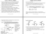
Design procedure for a small signal amplifier: 

1. List the specifications such as frequency, power gain, NF, etc. 

2. Choose a device --- very critical step. 

3. Measure S-parameter and noise parameters of the device (or 

obtain from the vendor) for the conditions specified (for the 

hybrid design). 

4. S-parameters and noise parameters from the foundry (for MMIC 

design). 

5. Study the Min., Max., and variations of the device parameters. 

6. Check the stability conditions. 

7. Plot constant gain and constant noise figure circles on the same 

Smith chart. 

ELEC518, Kevin Chen, HKUST 1 

8. Compute maximum power 

gain for the amplifier. 

9. Choose a source power gain 

circle to intercept with the noise 

circle. 

10. Design the input and output 

impedance matching network 

values --- another crucial step! 

11. Realize the matching 

networks based on the 

application at hand. 

12. Whenever possible, use good 

CAD tools for accurate design 

predictions. 


Narrow band amplifiers: typically have bandwidth less than 10% 

of the center frequency. Most of the amplifiers designed for 

portable communication amplifiers fall in this category. 

I. Maximum power gain design 

1. Determine the source and load impedances from the 

reflection coefficients data for the maximum power gain 

provided by the vendor. These values are taken at the center 

frequency for the amplifier. 

2. Realize the matching elements to transform the source and 

load impedances to 50 Ω. 

II. 

Low-noise amplifier design 

1. Determine the source impedance from the reflection 

coefficients data for minimum noise figure provided by the 

vendor. The load impedance is designed for the maximum 

power gain. These values are taken at the center frequency 

for the amplifier. 

2. Realize the matching elements to transform the source and 

load impedances to 50 Ω. 


ELEC518, Kevin Chen, HKUST 4

Broadband Transistor Amplifier Design: Balance Amplifiers 

III. Special considerations for monolithic RFIC circuit design: 

1. Try to minimize the space taken by passive components to 

reduce the die size (and therefore the cost). 

2. Element values limited by planar process. 

3. The design must be tolerant to the expected process 

variation of the active device parameters due to the lack of 

tuning capability. 

4. RFIC/MMIC design requires “yield-driven” approach, 

compared to the “performance-driven” approach of the 

hybrid IC design. 


Challenges for broadband transistor amplifiers: 

• Conjugate matching will give maximum gain only over a 

relatively narrow bandwidth. 

• Designing for less than maximum gain will improve the gain 

bandwidth, but the input and output ports of the amplifier will be 

poorly matched. 

• Gain rolloff of |S 21 | at a rate of 6 dB/octave. 

Some common approaches to design broadband amplifiers: 

• Compensated matching networks: frequency response of the 

matching network can compensate the gain rolloff in |S 21 | . 

• Negative feedback: flatten gain response, at the expense of gain 

and noise figure. 

• Balanced amplifiers: good matching, but the design is more 


complicated. 

Broadband Transistor Amplifier Design 

• Microwave transistors typically are not well matched in 

broadband amplifiers. 

• Broader bandwidth can be obtained at the expense of gain and 

complexity. 

Common approaches to achieving broader bandwidth 

Balance Amplifiers 

Two amplifiers having 90 o couplers at their input and output can 

provide good matching over an octave bandwidth, or more. The 

gain is equal to that of a single amplifier, however, and the design 

requires two transistors and twice the DC power. 

• Compensated matching networks: matching networks can be 

designed to compensate for the gain rolloff in S21. 

• Resistive matching networks: better matching with a loss in gain 

and increase in noise figure. 

• Negative feedback: negative feedback can be used to flatten the 

gain response of the transistor at the expense of gain and noise 

figure. 



How is the input and output mismatch improved in 

Balance Amplifiers? 

The input at each amplifier is given by 

1 V 

2 

j 

2 V 

+ VA 

1 

= 

+ − + 

1+ 

V B 1 

= 

1 

The output is given by 

− − j + 1 

V2 

= VA2 

+ V 

2 2 

− j + 

= V1 

( GA 

+ GB 

) 

2 

+ 

B2 

− j 

= GAV 

2 

+ 

A1 

1 

GBV 

2 

+ 

B1 


+ 

S 21 of the overall amplifier is 

Overall gain of the balanced amplifier is the average of the 

individual amplifier. 

The total reflected voltage at the input can be written as 

V 

= 

− 

1 

1 − − j 

= VA 

1 

+ V 

2 2 

1 + 

V1 

( ΓA 

− ΓB 

) 

2 

− 

B1 

= 

− 

V2 

− j 

S = = ( G A 

+ G 

V + 

2 

21 B 

1 

1 

ΓAV 

2 

+ 

A1 

− j 

+ ΓBV 

2 

1 

S 11 of the overall amplifier is ( ) 

S 

V 

+ 

B1 


1 

− 

11 

= = ΓA 

− ΓB 

V + 

1 2 

S11 is small as long as the two amplifiers are close in performance. 

) 

Advantages of balanced amplifiers 

Performance and Optimization of a Balanced Amplifier 

Pozar, p. 834-835. 



Distributed Amplifiers 

Operating principle 

• Old idea getting a new life. 

• Bandwidth in excess of a decade are possible, with good input 

and output matching. 

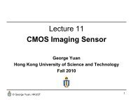
Configuration of an N-stage distributed amplifier. 


• The input signal propagates down the gate line, with each FET 

tapping off some of the input power. 

• The amplified output signals from the FETs form a traveling 

wave on the drain line. 

• The propagation constants and lengths of the gate and drain lines 

are chosen for constructive phasing of the output signals. 

• The termination impedances on the lines serve to absorb waves 

traveling in the reverse directions. 

• The gate and drain capacitances of the FET effectively become 

part of the gate and drain transmission lines, while the gate and 

drain resistances introduce loss on these lines. 

• Distributed amplifiers are also know as the traveling wave 

amplifiers (TWAs). 


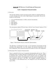
Analysis: separate loaded transmission lines for gate and drain 

Transmission line circuit for the drain line. 

Transmission line circuit for 

the gate line. 

Equivalent circuit of a single 

unit cell of the gate line. 



Gate transmission line analysis 

Z 

= jω 

L g 

Y 

= jωC 

g 

jωCgs 

/ lg 

+ 

1+ 

jωR C 

New characteristic impedance of the gate line is 

Z 

g 

= 

The attenuation is: 

γ = α + jβ 

= 

g 

g 

g 

Z 

Y 

ZY 

= 

= 

C 

g 

L 

g 

+ C 

gs 

/ l 

g 

⎡ 

jωLg 

⎢ jωC 

⎢⎣ 

g 

i 

gs 

jωCgs 

/ l 

+ 

1+ 

jωR C 

i 

g 

gs 

⎤ 

⎥ 

⎥⎦ 

Drain transmission line analysis 



Gain of a distributed amplifier: 



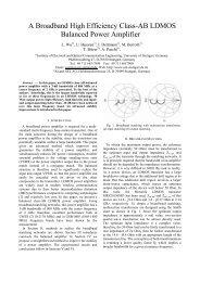
Power Dividers and Directional Couplers 

• Passive components used for power division or power 

combining 

• In the form of three-port (T-junction) networks and fourport 

(directional) networks 

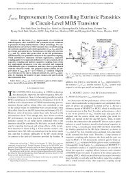
Reference: Y. Ayasli, et al. 

IEEE Trans. Microwave Theory and 

Techniques, vol. 30, pp. 976-981, July 

1982. 


Basic Properties of Dividers and Couplers 

Three-Port Networks (T-Junctions) 

It would be useful to have a passive lossless network that 

divides input port power at any port between the other 

two ports while being matched at all three ports. This 

would require the network to be matched, lossless and 

reciprocal. 


Network S-matrix 

(1) Matched S ii = 0 

(2) Lossless Unitary [S] 

(3) Reciprocal 

Symmetric [S] 

0 S 12 S 13 

[S] = S 21 0 S 23 

S 31 S 32 0 

This matrix can satisfy (1) 

and (3), but not (2). 

Therefore, using “normal” lossless components such as 

transmission lines, capacitors and inductors it is impossible to 

construct a 3-port network matched at all 3 ports. 

Need to relax one of the restrictions. 

A. For a nonreciprocal 3-port network (S ij ≠ S ji ), using 

anisotropic materials (such as ferrite), all ports can be 

matched and a circulator is created. 

Two Types of Circulators 

(1) Clockwise circulation 

0 0 1 

[S] = 1 0 0 

0 1 0 

it rotates power from port 1->2, port 2->3 and port 3->1. 

(2) Clockwise circulation 

0 1 0 

[S] = 0 0 1 

1 

1 0 0 

it rotates power from port 1->2, port 2->3 and 

port 3->1. 

1 

2 

3 

2 

3 



Applications of Circulators: 

• Protects a power amplifier from output mismatch. 

• Allows a transmitter and receiver to share an antenna. 

B. For a lossless and reciprocal 3-port network (S ij = S ji ), 

but with only two ports matched. 

0 S 12 S 13 

[S] = S 12 0 S 23 

S 13 S 32 S 33 

The requirement for unitary 

matrix leads to 

0 e jθ 0 

[S] = e jθ 0 0 

0 0 e jφ 

Totally mismatched 


C. For a reciprocal and all-matched 3-port network (S ij = 

S ji ), but with lossy components. 

This is the case of the resistive divider. A lossy 3-port 

network can be made to have isolation between its output 

ports. 

Four Port Networks (Directional Couplers) 

Pozar’s book shows that a matched, reciprocal, lossless four-port 

network is possible, and that it has directional coupling between 

pairs of ports. 

There are two possible forms of [S] for a directional coupler, one 

with outputs differing by 90° in phase and the other with outputs 

differing by 180° in phase. Any 90° coupler can be made into a 

180° coupler by adding a 90° transmission to one port, and vice 

versa. 


Input 

Isolated 

1 

4 

⎡ 0 

⎢ 

α 

[ S] 

= ⎢ 

⎢ jβ 

⎢ 

⎣ 0 

90° 

Coupler 

α 

0 

0 

jβ 

0 

0 

α 

2 

3 

jβ 

90° 

0 ⎤ 

jβ 

⎥ 

⎥ 

α ⎥ 

⎥ 

0 ⎦ 

Output 

Coupled 

2 2 

α + β = 1 

Σ 

∆ 

1 

4 

⎡0 

⎢ 

α 

[ S] 

= ⎢ 

⎢β 

⎢ 

⎣0 

180° 

Hybrid 

− β 

180° 

Output 

Output 


α 

0 

0 

2 

3 

β 0 ⎤ 

0 − β 

⎥ 

⎥ 

0 α ⎥ 

⎥ 

α 0 ⎦ 

Any 90° coupler can be made into a 180° coupler by adding a 

90° transmission to one port, and vice versa.. The 90° coupler is 

referred to as a quadrature hybrid, and can be created using directly 

connected branch lines between two transmission lines or by means 

of coupled transmission lines. 

Input 

Isolated 

1 

Zo 

4 

λ/4 

Zo/¦2 

2 

λ/4 

3 

Output 

Output 

Coupled 

A branch-line coupler A coupled-line 

directional coupler 

Coupling, Directionality and Isolation 

Input 

Coupling = C = 10log(P1/P3) = -20logβ dB 

Directivity = D = 10 log (P3/P4) = 20logβ/ |S 14 |dB 

Isolation = I = 10log(P1/P4) = -20log |S 14 |dB 

I= D + C dB 

Isolated 

Through 


Resistive Divider 

If we relax the requirement for zero loss, 

we can realize a matched, reciprocal 

power divider. 

Such a divider 

can be realized 

by connecting 

three Zo 

transmission 

lines to a star 

circuit consisting 

of three resistors 

R = Z o /3. 

An equal-split three-port 

resistive power divider. 

The impedance looking into the resistor 

followed by the output line, is 

Z0 4Z 

Z = + Z0 

= 

3 3 


0 

The input impedance of the divider is 

Z 

3 

2Z 

3 

0 0 

Z in 

+ = 

= matched 

Since the network is symmetric from all three ports, the 

output ports are also matched. 

Output Power 

The output voltage from port 2 and 3 are, 

Z 

0 

V1 

V 

2 

= V3 

= 

2 

Thus, S 21 = S 31 = S 23 = 1/2, which indicates -6 dB below 

the input power level. We have 

⎡0 

1 1⎤ 

1 

1 

⎢ ⎥ Port 2 and 3 are 

[S] 

= 1 0 1 

P2 = P3 

= Pin 

2 ⎢ ⎥ not isolated. 

4 

⎢⎣ 

1 1 0⎥⎦ 

power 


The Wilkinson Power Divider 

Motivation: to solve the problem of output isolation 

The Wilkinson power divider is a three-port that has all ports 

matched with isolation between the two output ports. 

An equal-split Microstrip Wilkinson Equivalent circuit 

power divider 

The Wilkinson power divider can be made to give arbitrary 

power division. But an equal-split one is used here for 

analysis. 


Features of the Wilkinson dividers 

1. By choosing the impedance of the λ/4 lines to be 2 Z o , the 

matched output loads Z L = Z o are transformed to 2Z o so they can be 

placed in parallel to equal 2Z o /2 = Z o creating a matched condition at 

the input port. 

2. Any mismatched power returned from a load at either output port is 

divided equally between the load on the input port (the generator 

source impedance, presumed to be Z g = Z o ) and the resistor R. 

3. None of the reflected power from a mismatched load is dissipated 

in the other load, so the output ports are isolated (S 23 = S 32 = 0). 

When the Wilkinson power divider is driven at port 1 and the 

outputs are matched, no power is dissipated in the resistor. Thus the 

divider is lossless when the outputs are matched; only reflected 

power from ports 2 or 3 is dissipated in the resistor. Since S 23 = S 32 

= 0, ports 2 and 3 are isolated. 


S-parameters of a Wilkinson divider 

S = 0 

0 

11 

S = S 

22 33 

= 

The (4-port) Directional Couplers 

• A fraction of a wave 

traveling from port 1 to port 

2 via the transmission line 

1-2 is coupled to port 3, but 

not to port 4. 

• A fraction of a wave 

traveling from port 2 to port 

1 is coupled to port 4, but 

not to port 3. 

• The same coupling exists in 

transmission line 1-2 for 

waves traveling on line 4-3. 

S 

e o 

1 1 

12 

= S21 

= 

e o 

V2 

+ V S23 = S32 

= 0 

2 

= − j / 

V 

2 

+ V 

Symbols for directional couplers. 


Recalling the definition of Coupling, Directivity and 

Isolation factors. 

C and D can be measured directly, but the 

Coupling = C =10log(P 1 /P 3 ) power level at the coupled ports (3 and 4) 

may be small enough to make this 

Directivity = D = 10 log(P 3 /P 4 ) difficult, particularly if the signal coupled 

Isolation = I = 10log(P 1 /P 4 ) from the input to reverse output port 4 is 

masked by a reflected wave from an 

imperfectly matched load at port 2. 

The Quadrature (90 O ) Hybrid Directional 

Couplers 

• A 3 dB directional coupler with a 90 o phase difference in the 

outputs of the through and coupled arms. 

• Exist in the form of branch-line, coupled line and or Lange 

(interdigitated). 


Brach-Line Couplers 

Highly symmetric 

A branch-line coupler in 

normalized form 

B = 0 1 

(port 1is matched) 

j 

o 

B2 

= − (half - power, - 90 phase shift from port 1 to 2) 

2 

B3 = − 

1 o 

2 

(half - power, -180 

phase shift from port 1 to 3) 

⎡0 

⎢ 

−1 

j 

The [S] matrix is given by [ S] 

= ⎢ 

2 ⎢1 

⎢ 

⎣0 

A practical microstrip quadrature 

hybrid prototype. 

Some practical design issues: 

1. Limited bandwidth: due to the nature 

of quarter-wave line. Multisection design 

will help. 

2. The effect of discontinuity at the 

junctions: shunt arms are usually 

lenghthened by 10 o -20 o . 

B = 0 4 

(no power to port 4) 



j 

0 

0 

1 

1 

0 

0 

j 

0⎤ 

1 

⎥ 

⎥ 

j⎥ 

⎥ 

0⎦

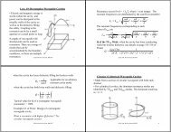
Coupled Line Theory 

Various geometries 

Edge-coupled stripline Broadside-coupled stripline 

Edge-coupled microstrip line. 

Even mode excitation: E-field symmetric about the center line 

C 12 is opencircuited 

C e =C 11 = C 22 , 

assuming the 

two strips are 

identical in size 

and location. 

Z 

L 

LC 

e 

0e = = = 

Ce 

Ce 

1 

vC 

Odd mode 

where v is the propagation velocity on the line. 

excitation C o =C 11 + 2C 12 = C 22 + 2C 12 

e 

, 

Equivalent circuit 


Z 

0 e 

= 

1 

vC 

o 

Voltage null 


Tight Couplers: The Lange Couplers and Ring 

Hybrid Couplers 

• Coupled-line couplers are not suitable to achieve coupling factors of 

3 dB or 6 dB, due to the loose coupling. 

• Tight coupling can be achieved by the special layout of the coupled 

lines, so that the fringing fields at the edge of the lines can contribute 

to the coupling. 

The Lange Couplers: 

The interdigitated Lange coupler The unfolded Lange coupler 


The Lange couplers has the following features: 

• There is a 90 o phase difference between the output lines (ports 2 and 3) 

• Difficult to fabricate the bonding wires due to the narrow spacing between 

the lines. 

The 180 o Hybrid 

• The two outputs are either in phase 

or with a 180 o phase difference. 

• A signal applied to port 1 is evenly 

divided into two in-phase 

components at port 2 and 3, with port 

4 isolated. 

• A signal applied to port 4 is equally 

split into two out-of-phase 

components at port 2 and 3, with port 

1 isolated. 

⎡0 

⎢ 

− j 1 

[ S] 

= ⎢ 

2 ⎢1 

⎢ 

⎣0 

−1 

0 ⎤ 

−1 

⎥ 

⎥ 

1 ⎥ 

⎥ 

0 ⎦ 


1 

0 

0 

1 

0 

0 

1

• When operated as a combiner, with inputs at ports 2 and 3, the sum of 

the inputs will be formed at port 1 (the sum port), while the difference 

will be formed at port 4 (the difference port). 

Ring Hybrid (rat-race): a typical 180 o Hybrid 

Port 3 

Port 1 

Port 4 

Port 2 

Similar to branch-line coupler. Can be easily constructed in 

planar (microstrip or stripline) form. Read pp. 403-407 of Pozar.

Lecture 6: Microwave Amplifiers (3)

You also want an ePaper? Increase the reach of your titles

Delete template?

Save as template?