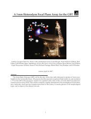
Spectral-line Observations with the GBT K-band Focal Plane Array

Spectral-line Observations with the GBT K-band Focal Plane Array
DRAFT: June 19, 2008
D.J. Pisano
1. The GBT K-band focal plane array
The GBT K-band focal plane array (KFPA) is a 7-beam array of receivers that is due to be completed
by 2010. It will operate over a frequency range of 18-26.5 GHz and have T rx

– 2 –
1 0 ), and H 2 O masers in the star-forming region B1-IRS. They found maser emission peaking at ∼15
mJy (although previous epochs had emission 100 times brighter). The NH 3 (1,1) emission peaks at
T MB ∼4 K for the main line and ∼1 K for the satellite lines. CCS peaks at ∼0.7 K.
• Kaifu et al. (2004) surveyed TMC-1 using the 45-m Nobeyama telescope. They found lines of HC 3 N,
c-C 3 H 2 , HC 5 N, C 4 H, HC 7 N, CCS, CCCS, and NH 3 that are all detectable with 60 seconds on-source.
• Pillai et al. (2006) studied NH 3 (1,1) and (2,2) in nine infrared dark clouds. They found peak T MB
values of 2-4 K for the main line of NH 3 (1,1) and 0.5-1 K for the hyperfine transitions. For the (2,2)
transition, the peak T MB is ∼0.5-2 K. FWHM linewidths were of order 1 km s −1 .
• Rosolowsky et al. (2008) used the GBT to survey NH 3 (1,1), (2,2), and CCS in dense cores in the Perseus
molecular cloud spanning a range of environments from clusters to isolated star-forming regions to nonstar-forming
regions. T MB for NH 3 (1,1) ranges from ∼0.5 - 5 K, and ∼0.2-1 K for NH 3 (2,2). For CCS
the peak T MB ranges from ∼0.1 - 1 K. For all lines σ v ∼0.2 km s −1 .
• Bell et al. (1993) observed W51, a complex of molecular clouds and star-forming regions between 17.6-
22.0 GHz with the Green Bank 140 ft telescope. The only lines they identified with T A ≥0.1 K were
hydrogen recombination lines, NH 3 (9,6), and C 3 H 2 .
• Rathborne et al. (2008) observed NH 3 (1,1), (2,2), CCS, and HC 5 N(9,8) towards 46 dense cores in the
Pipe nebula with the GBT down to a 1σ rms of 0.01-0.07 K. Peak T ∗ A values for NH 3(1,1) ranged
from 0.1-4 K with the satellite lines visible only in the brightest spectra. For NH 3 (2,2), T ∗ A ranged
from 0.06-1.37 K. Velocity dispersions for NH 3 were about 0.1-0.2 km s −1 . CCS was detected from
fewer cores, but was sometimes stronger than NH 3 (1,1). The peak T ∗ A ranged from 0.06-0.78 K. For
HC 5 N(9,8), only 4 cores had detectable emission with 0.27-0.58 K peak T ∗ A .
• Longmore et al. (2007) observed NH 3 (1,1), (2,2), (4,4), and (5,5) towards hot molecular cores with
methanol maser emission; the sites of massive star formation using the ATCA. NH 3 (1,1) lines had
peak fluxes of 0.2-0.4 Jy, with the satellite lines at 0.1-0.2 Jy. The NH 3 (2,2) line generally peaked at
0.05-0.1 Jy, and the NH 3 (4,4) and (5,5) lines peaked at 0.05-0.1 Jy.
• GBT observations of SgrB2 (N-LMH) by Hollis et al. (GBT07A-051) show that this star-forming, giant
molecular cloud complex has quite different emission ratios than other regions. For example, they find
that the main lines of NH 3 and CCS are in absorption instead of emission. Other transitions of NH 3
and other molecules (such as HC 3 N, HNCO, CH 3 OH, and OCS) are seen in emission and are easily
bright enough to detect with the observing parameters above (Remijian 2008, private communication).
Some observers may also use the GBT KFPA for extragalactic observations of NH 3 , H 2 O masers, or
other lines. These may or may not involve mapping; here are a few examples:
• Ott et al. (2005) used the ATCA to observe NH 3 (1,1), (2,2), (3,3), and (6,6) in the galaxy NGC 253.
Peak fluxes ranged from 10 to 50 mJy over a 30 ′′ ×5 ′′ beam with a total FWHM linewidth of ∼200 km
s −1 .
• Braatz & Gugliucci (2008) used the GBT to search for water maser emission from the nuclei of nearby
galaxies. Such emission was found in 8 galaxies ranging from 16-138 mJy. Hagiwara (2007) used the
VLA to search for low luminosity water masers from nearby star-forming galaxies. A number of masers
with peak fluxes ∼50 mJy in M 82, M 51, and NGC 4051 (and there are similar examples in other
galaxies studied by other authors).

– 3 –
The main benefit of the KFPA is its ability to map large areas of sky rapidly. Given the typical line
strengths listed above, the majority of the mapping with the KFPA will be done of star-forming regions and
molecular clouds in the NH 3 (1,1) line. However, for some objects, NH 3 (2,2), CCS, or other, more complex
molecules may be able to be mapped with integration times of 1-2 minutes per pixel. For this science, source
sizes range from the GBT beamsize (33 ′′ ) to the entire Galactic plane (hundreds of square degrees). We
expect that most mapping observations will be of individual star-forming cores and and infrared dark clouds
(IRDCs) to complexes of these objects. These complexes will range from a few to 10s of arcminutes in size
(e.g. Pillai et al. 2006; Rosolowsky et al. 2008, ; Friesen et al. 2008, in preparation; Morgan et al. 2008, in
preparation).
For observations of NH 3 that seek to derive temperatures and densities of the molecular gas and search
for signatures of inflow or outflow (e.g. Longmore et al. 2007), the high spectral resolution cited above are
necessary for resolving the NH 3 lines. Some observations can use coarser spectral resolution, e.g. 6.1 kHz,
where the lines do not need to be fully resolved.
For chemistry surveys, the KFPA can still be used in a non-mapping mode (to be described below). For
extragalactic targets, NH 3 will be detectable with much deeper observations, as will H 2 O maser emission.
3. Possible KFPA observing modes
There are a number of possible observing modes for the KFPA, but they broadly break down into
mapping and single-pointing modes. In general, existing Astrid scan types and GBTIDL reduction procedures
should be sufficient for data acquisition and reduction. There are a number of features that could be added
to existing routines, however, to improve observing efficiency and improve data quality. For example, RFI
can be rejected automatically if all beams show a spike at the same time. Redundant observations of the
same sky position with multiple beams will also improve the quality of the final maps.
3.1. Mapping with the KFPA
3.1.1. On-the-fly mapping
On-the-fly (OTF) mapping has become the standard method for mapping large areas of sky quickly and
efficiently (e.g. Holland et al. 1999; Barnes et al. 2001; Jackson et al. 2006; Mangum et al. 2007). Because of
the power of the KFPA to map large areas, this is likely to be the primary mode of operation for the KFPA
and the most important mode for development of a pipeline.
Independent of the feed configuration, the most common approach is to scan the array along lines of
constant RA and Declination (Barnes et al. 2001) or Galactic latitude and longitude (Jackson et al. 2006)
making a raster and, sometimes, a basket-weave map. Consecutive stripes of the map are offset at the
Nyquist spacing. OTF maps have to have some “OFF” position for calibration. This can be provided either
by a separate, distinct “OFF” position from the map (Jackson et al. 2006) or using line-free regions of the
map (Barnes et al. 2001) or, in the cases where emission fills the map (e.g. for Galactic HI), frequencyswitching
is used (e.g. Lockman et al. 2008). For ammonia mapping, the emission will generally fill the map,
so frequency-switching will be used. For other molecules a dedicated “OFF” position or the blank areas of
the map can be used. Other scanning patterns may be more efficient in terms of overheads, for example
MUSTANG uses a “billiard ball” trajectory, but the basic approach for reduction is independent of the exact

– 4 –
trajectory used. I will explore alternative trajectories and their associated mapping efficiency in a future
memo.
For the KFPA on the GBT, we can use existing mapping procedures present in Astrid: RALongMap,
RALongMapWithReference, DecLatMap and DecLatMapWithReference. Because we can not rotate the
KFPA feed pattern, observers will want to map the region of interest by Nyquist sampling with each beam
of the array. This has the drawback of providing a reduced sensitivity border around the object being
mapped and higher overhead. This region could be used to improve the calibration of the map, however.
For frequency-switched data and if the noise diode is fired while scanning, then the data rate will have to be
higher so that all phases of switching sample closely the same position on the sky (within a fraction of the
beamwidth).
For reducing OTF data, the GBTIDL routines also already exist to reduce most of this data. For
frequency-switched data, each beam and polarization can be separately reduced using getfs. For data taken
with an “OFF” position, then getps or getsigref can be used. It is only the scenario where an observer wishes
to use the line-free portion of the map as an “OFF” position that GBTIDL can not currently handle the
calibration. This approach was used by HIPASS (Barnes et al. 2001) and other surveys using the Parkes
20cm multibeam (e.g. Pisano et al. 2007) as well as the ALFALFA survey (Giovanelli et al. 2005), although
the details on the reduction are not yet published]giovanelli05. So the calibration and bandpass correction
should not require any new algorithm development.
There are many algorithms available for gridding OTF data. Currently for GBT observations, GBTIDL
is used for the calibration and bandpass calibration and then the data is exported to AIPS where the task
SDGRD is used to make an image. For Parkes and some ALFA data, livedata and gridzilla are used.
The data rate for OTF mapping with the 7-pixel KFPA will require dumping 14 samples (7 beams,
2 polarizations) for each phase of a frequency-switch and of the noise diode firing. For a 33 ′′ beam, that
means we will need to dump every 13 ′′ . For the GBT Spectrometer, we can switch at a maximum rate of
95 Hz for 4 phase switching (cal on and cal off for signal and reference frequencies) and with a minimum
hardware-limited dump time 1 of 1.44 seconds to a local disk (although typical dump times are ∼2 seconds
for an NFS-mounted disk). Since the minimum dump time is only 40% less than the typical dump time, we
will just consider the latter. A 2 second dump time yields a scanning rate of 6.5 ′′ s −1 . These rates are much
less than the slew speed, so we will not run into any hardware limits for mapping.
If we have either 12.5 MHz or 50 MHz bandwidths, then we will have no more than 16384 channels per
sampler (for 3 level sampling). With only 4 phases per integration, then we will have 65 kB per integration.
For a 2 second integration, this is 1.8 MB/s. Using the minimum dump time, the data rate is 40% higher.
If the noise diode is not fired during the mapping observations or frequency-switching is not used, then
the data rates would be halved. If, however, the switching rate is increased, then the data rate would be
proportionally higher. A new backend that can fully sample the 1.8 GHz IF bandwidth will have a data rate
that is no more than 144 times (1.8 GHz/12.5 MHz) higher for the same spectral resolution. For increased
spectral resolution, the data rate will increase proportionally. For a 61-pixel array, the data rate would
increase by another factor of 9. Finally, if the entire receiver bandwidth is sampled, then the data rate is no
more than 576 times higher (8 GHz/12.5 MHz) for the same spectral resolution. All told, this could result
in data rates for a 61-pixel FPA sampling the full 8 GHz bandwidth of ∼10 GB/s. While all of this data
need not be saved on disk, it is still beyond our current capabilities.
1 The minimum dump time for the Spectrometer is 0.09× N phases × N quadrants .

– 5 –
For a map size of 3 ′ ×3 ′ (26 beams) with a total integration time of 1 minute per beam, the 7-pixel
KPFA will produce 406 MB of data with 2 second integrations. If the map is of a typical IRDC (about
12 ′ ×12 ′ in size), then a total of 6.5 GB of data will contribute to a map.
3.1.2. Jiggle mapping
For mapping sources smaller than the array, we can either do a very small OTF map using the same
approach as described above, or we can use a jiggle map similar to the technique used by SCUBA (Holland
et al. 1999). For a single SCUBA array, there is a 16 point pattern that the array is cycled through. Each
point is offset by half a beamwidth from the neighboring point. For SCUBA, the telescope is nodded to an
“OFF” position each cycle while chopping occurs throughout the observing. For the KFPA, the feed spacing
is larger than for SCUBA so the equivalent pattern would have 36 pointings. Because the atmosphere is
more stable at 22 GHz than at 450 µm, the “OFF” position would not need to be visited as often by KFPA
as for SCUBA. If frequency-switching is used, then no distinct “OFF” position would be needed.
The weakest aspect of a jiggle map is that the GBT will have to slew and then dwell at each position
leading to larger overheads. This overhead could be reduced by using the subreflector to move between
positions, but it will still be larger than for an OTF map. Using the subreflector for this motion would also
limit the variations of the atmosphere between pointings. The 36 point cycle should be done on a short
enough time period that field rotation is not large. This observing mode could be mimicked by an OTF map
with an appropriate scanning rate.
A jiggle map could be made using a simply modified form PointMap or PointMapWithReference. Reduction
could be done in the same manner as for an OTF map.
3.2. Single-pointing modes
While mapping is likely to be the most common mode of observing for the KFPA, it is likely that the
performance of the array will be at least as good as the existing K-band receiver. Therefore, the KFPA may
replace this receiver for observations of point sources as well. There are a number of observing modes that
will be used for observing point sources with the KFPA.
3.2.1. Traditional switching
The KFPA will be able to use traditional observing modes, such as position-switching and frequencyswitching.
This could be done using all 7 (or 61) beams or a subset of beams (1,2, or 4). Position-switching
would be used for sources that are extended with respect to the array, but which the observer does not wish
to map (for astrochemistry surveys, for example). Frequency-switching could be used for either extended
sources or point sources located in a single beam. Because of field rotation over time, the outer beams will
smear into an annulus over time so minimal information will be available about the distribution of emission
from a source.
Observations would be carried out using standard Astrid scan types such as Track and OnOff (or OffOn)
and reduction in GBTIDL such as getfs and getps.

– 6 –
Single pixel operation will be possible for VLBI observing as well.
3.2.2. “MX” mode
For point-sources, an array provides a powerful mode for improving observing overhead and the signalto-noise
delivered in a given amount of observing time as well as data quality. This mode has been used
by the Parkes multibeam for point source observations and is called “MX” mode. It is a generalization of
standard dual-beam, nodding observation as done currently at the GBT. For the 7-pixel KFPA, an observer
would point each beam in turn at the source while the other beams observe an “OFF” position. This “OFF”
position would be different for each beam and would rotate with time. Long dwell times for each beam are
possible, but, in general, observers will want this to be reasonably short (of order one minute) to minimize
rotation and variations in the atmosphere.
This mode provides six times the integration time in the “OFF” position as in the “ON” position yielding
improved signal-to-noise. Because “OFF” observations will generally bracket the “ON” observations, so the
background subtraction should also be improved. For the 61-pixel KFPA, it is likely that only a subset
of beams would be used. Switching between beams could be done by slewing the telescope or tilting the
subreflector. To carry out these observations generalized forms of the Nod and/or SubBeamNod procedures
will need to be developed for multiple beam (greater than 2) receivers. To reduce the data, a change in
labels will be needed for GBTIDL routines to cope with multiple “OFF” beams and positions. Otherwise,
getnod or Ron Maddalena’s getSubrnod should be able to reduce the data with minimal changes.
3.3. Continuum Observing
There are plans to use the KFPA for continuum and polarization observations. While these observing
modes are not the primary science drivers, we expect that the KFPA will be used and be useful for this
science. It is likely that continuum observing with the KFPA and subsequent data reduction will utilize a
similar strategy as is used for the GALFACTS project with the ALFA multibeam.
3.4. Feed Layout
Some FPAs have been packed in a hexagonal configuration (like SCUBA, the Parkes multibeams, and
ALFA), while other FPAs have been rectangularly packed (like SEQUOIA, BEARS, and HARP). Is there a
preferred configuration for the KFPA given its anticipated usage?
A hexagonally packed array places the feeds as close together as physically possible. For the KFPA,
this corresponds to a 3 beamwidth spacing at 24 GHz. As such, this maximizes both the number of feeds
we can fit in a dewar and the amount of area covered by the array in a single-pointing. The dense packing
may make it more difficult to access the front-end electronics for maintenance, however this does not appear
to be a concern for KFPA and is certainly not an issue for the 7-pixel array. Finally, with a hexagonally
packed array the telescope can be scanned at an angle of 19 ◦ to any of the long axes of the array to produce
tracks that are spaced at 1 beamwidth instead of the 3 beamwidth physical spacing for the KFPA. Since the
KFPA will not have a feed rotator, it will not be possible to scan at this angle most of the time, but we can
scan at close to this angle with the correct array configuration. This is less important for the full 61-pixel

– 7 –
array due to the redundancy of that configuration.
A rectangular packed array is a simpler geometry and provides more room for access to front-end
electronics. It is not as densely packed as a hexagonal configuration and there is no magic scanning angle.
This has not been a problem for other arrays, even those without feed rotators (e.g. Jackson et al. 2006), but
does require more rapid sampling when scanning. Clever scanning algorithms may also mitigate this problem.
It is not evident, however, what advantages beyond simplicity a rectangularly packed array provides.
3.5. Possible alterations to existing systems
Is there additional metadata needed to make data reduction possible or more efficient? Are there any
hardware-related upgrades that would be necessary or helpful? Finally, what additional features could be
added to ASTRID, SDFITS, or GBTIDL that would exploit the multibeam nature of the KFPA? This
section summarizes some of the answers to these questions.
Beyond the plans for a more detailed database for calibration (including vector T cal values, for example)
and weather-related information (like the opacity), the main alteration of existing software will involve the
proper accounting of more than two beams. Currently, the SDFITS filler and GBTIDL can deal with simple
position-switched and nodding data from dual beam receiver. However, having numerous beams (up to 61)
requires keeping track of many “OFF” positions. If the subreflector is used to switch between beams, then
the current system of assigning a flag based on whether the subreflector is moving or aligned with beam 0
or 1 will need to be expanded to cope with up to 61 beams. In addition, particularly for a 61 beam array,
the aperture efficiency will vary between beams requiring different aperture efficiencies to be used for each
beam.
The above observing modes should be simple generalizations of current ASTRID scan types. New
wrappers should probably be written to allow easier use of a OTF map or a jiggle map for the KFPA, but
the current scan types should work. The “MX” mode will require a new scan type in ASTRID. It may
exploit the subreflector, which can be done using the SubMotion object (or a variation on it).
For GBTIDL, existing reduction algorithms should work for all observing modes, except for “MX” mode.
For “MX” mode, there will need to be an alteration to the code to average multiple “OFF” scans and use
those for calibration and bandpass correction. These scans could be combined either with a straight average
or some sort of median or minmax combination to mitigate RFI and cope with bad or missing integrations.
The “MX” mode will be necessary for calibrating the array, since each beam will need to observe a known
flux calibrator to derive vector T cal values.
Currently, imaging for GBT mapping data is done via AIPS. This approach should still work for the
7-pixel KFPA if AIPS can cope with the data volume. The data volumes could be prohibitively large for
this approach to work for the 61-pixel KFPA.
There is currently no statistical flagging available in GBTIDL. The KFPA is well-suited to some simple
flagging and calibration tasks that exploit the redundancy of a multibeam system. For example, if all beams
experience a sudden change in their power levels, then the source is likely to be RFI and is not astronomical.
Additionally, atmospheric variations will be (mostly) common between beams and slowly varying. There are
a number of instruments that exploit this information for improved atmospheric removal. For example, this
is done with MUSTANG on the GBT. Finally, all beams should measure the same flux when observing the
same direction on the sky. This “basket-weaving” calibration can be used to improve the standard calibration

– 8 –
as is being done for the GALFACTS observations. This is not a necessary step, but may improve the data
quality for the KFPA. It may be particularly useful for removal of atmospheric variations.
4. Summary of Pipeline Priorities
What should the software priorities for pipeline development be? These have been discussed above, but
in priority order they are as follows:
1. The proper accounting of multiple beams by ASTRID, SDFITS, and GBTIDL.
2. The reduction and gridding of OTF data using existing GBTIDL routines.
3. The observing and reduction of “MX”mode observations.
4. Finally, the exploitation of multibeam observations for improved atmospheric removal, flagging, calibration
and analysis of the data.
In addition, development of continuum observing modes and data reduction is also necessary, but this
effort will likely be led by our collaborators in Calgary.
Thanks to Larry Morgan and Claudia Cyganowski for sharing their K-band observing experiences.
Thanks to Ron Maddalena, Mark Clark, and Bob Garwood for help with the data rate calculations.
Barnes, D. G., et al. 2001, MNRAS, 322, 486
REFERENCES
Bell, M. B., Avery, L. W., & Watson, J. K. G. 1993, ApJS, 86, 211
Braatz, J. A., & Gugliucci, N. E. 2008, ApJ, 678, 96
Giovanelli, R., et al. 2005, AJ, 130, 2598
De Gregorio-Monsalvo, I., Chandler, C. J., Gómez, J. F., Kuiper, T. B. H., Torrelles, J. M., & Anglada, G.
2005, ApJ, 628, 789
de Gregorio-Monsalvo, I., Gómez, J. F., Suárez, O., Kuiper, T. B. H., Rodríguez, L. F., & Jiménez-Bailón,
E. 2006, ApJ, 642, 319
Hagiwara, Y. 2007, AJ, 133, 1176
Holland, W. S., et al. 1999, MNRAS, 303, 659
Jackson, J. M., et al. 2006, ApJS, 163, 145
Kaifu, N., et al. 2004, PASJ, 56, 69
Lockman, F. J., Benjamin, R. A., Heroux, A. J., & Langston, G. I. 2008, ApJ, 679, L21
Longmore, S. N., Burton, M. G., Barnes, P. J., Wong, T., Purcell, C. R., & Ott, J. 2007, MNRAS, 379, 535

– 9 –
Mangum, J. G., Emerson, D. T., & Greisen, E. W. 2007, A&A, 474, 679
Ott, J., Weiss, A., Henkel, C., & Walter, F. 2005, ApJ, 629, 767
Pillai, T., Wyrowski, F., Carey, S. J., & Menten, K. M. 2006, A&A, 450, 569
Pisano, D. J., Barnes, D. G., Gibson, B. K., Staveley-Smith, L., Freeman, K. C., & Kilborn, V. A. 2007,
ApJ, 662, 959
Rathborne, J. M., Lada, C. J., Muench, A. A., Alves, J. F., & Lombardi, M. 2008, ApJS, 174, 396
Rosolowsky, E. W., Pineda, J. E., Foster, J. B., Borkin, M. A., Kauffmann, J., Caselli, P., Myers, P. C., &
Goodman, A. A. 2008, ApJS, 175, 509
This preprint was prepared with the AAS LATEX macros v5.2.