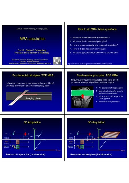
MRA acquisition

Annual RSNA meeting, Chicago, 2007 

How to do MRA: basic questions 

MRA acquisition 

Prof. Dr. Stefan O. Schoenberg 

Professor and Chairman of Radiology 

1. What are the different MRA techniques? 

2. What are the fundamental principles? 

3. How to increase spatial and temporal resolution? 

4. How to expand anatomic coverage? 

5. What are typical artifacts and how to avoid them? 

Department of Clinical Radiology and Nuclear Medicine 

University Hospital Mannheim, 

Medical Faculty Mannheim – University of Heidelberg, Germany 

http://www.ma.uni-heidelberg.de/inst/ikr/RSNA2007/MRAacquisition 

Fundamental principles: TOF MRA 

Inflowing, previously un-saturated spins (e.g. blood) 

produce a stronger signal than stationary spins 

Imaging plane 

Fundamental principles: TOF MRA 

Inflowing, previously un-saturated spins (e.g. blood) 

produce a stronger signal than stationary spins 

1. Pre-saturation of imaging plane 

2. Magnetization transfer pulse for 

background suppression 

3. Inflow of blood (90°angle to the 

imaging plane) 

4. Insensitive for inplane flow 

3D Acquisition 


k Slice 

k Slice 

RF 

α 

RF 

α 

Readout 

gradient 

k Readout 

Readout 

gradient 

k Readout 

Phase 

gradient 

Phase 

gradient 

Slab/Slice 

gradient 

Slab/Slice 

gradient 

k Phase 

k Phase 

Readout of k-space line (1st dimension) 

Readout of k-space plane (2nd dimension)


3D Acquisition: 3D Time-of-flight 

k Slice 

RF 

α 

Readout 

gradient 

k Readout 

k Readout 

Phase 

gradient 

Slab/Slice 

gradient 

k Slice 

Readout of k-space volume (3rd dimension) 

Fourier 

transform 

k Phase 

k Phase 

Readout of k-space volume (3rd dimension) 

3D Time-of-flight @ 3 Tesla 

Time-of-flight 3T versus 7T 

3 Tesla 7 Tesla 

ACA 

ACA 

MCA 

MCA 

MCA 

MCA 

CS CS 

CS CS 

post. CA 

post. CA 

PCA 

PCA 

PCA 

PCA 

Courtesy of Paul Finn MD PhD 

0.3mm x 0.3mm x 0.5mm 

Advantages / disadvantages of TOF MRA 

Contrast-enhanced MRA 

Advantages 

• No contrast media 

• Easy, completely noninvasive 

technique 

• Acquisition of 3D data 

sets possible 

Disadvantages 

• Long acquisition times 

motion artifacts 

• insensitive for slow 

flow and inplane flow 

• High background 

signal 

• High contrast due to contrast media application 

• Fast acquisition 

• High isotropic spatial resolution up to 1mm 3 

• Acquisition of 3D data sets 

• Minimum artifacts 

• Flow-independent b/o CM imaging of slow flow 

• State-of-the art in clinical routine for most applications

Application of contrast agents 

Technical principles of MRA 

Image 

Rawdata 



Image 

Rawdata 

Image 

Rawdata 


K-space bolus-timing 

Fourier- 

Transformation 

Fourier- 

Fast (< seconds) 


Fourier- 


Fourier- 

Slow (min) 


• Central parts of k-space CM bolus 

• Timing too late venous overlay 

• Timing too early poor vessel contrast 

• Determine time between injection and CM peak at the 

level of the target vessel 

test-bolus, automatic detection, fluoroscopic realtime 

visualization 

Image 

Rawdata

Timing is everything 

Test-Bolus technique 

Too early: “Ringing” artifact 

Too late: Venous overlay 

Courtesy of Martin Prince, MD PhD 

2000 

Automatic Gd Detection: Smartprep ® 

Start 

scanning 

Fluoroscopic assessment: Care Bolus®, Bolustrak®, 

MR Fluoroscopy® 

1800 

Integral of Echo Speed 

1600 

1400 

1200 

1000 

Start 

Injecting 

Gd 

Detect 

Gd 

2D Real time 

Visualization of contrast 

media arrival 

3D HR-MRA 

MIP 

800 

0 10 20 30 40 50 60 

Time (sec) 

Courtesy of Martin R. Prince, MD PhD 

Problem: delay (1-5 s) for online switch between fluoroscopy 

and MRA acquisition 

MRA: 

problem of 

spatial 

resolution 

Intravascular 

contrast agent 

(SHU 555C ) 

DSA 

0.3 x 0.3 mm 

MRA: Voxel size 

2.5 x 1.5 x 2 mm 


1.7 x 0.8 x 1.5 mm 


1.2 x 0.8 x 1.0 mm 

CE MRA – Increase of spatial resolution / 

decrease of scan time 

• (Zero Filling) 

• Partial Fourier Imaging 

• Elliptical centric acquisition 

• Parallel Imaging 

• Higher field strength 

• Radial Imaging

Acquired 

data 

Zero Filling 

k y 

k x 

128×128 128×128, zerofilled to 256×256 

Partial Fourier techniques 

• K-space is nearly symmetric 

• Acquisition of k-space parts with mirroring of the data 

number of phase-encoding steps ↓ acquisition time ↓ 

k y 

Zerofilled 

C 

B 

A 

k y 

256×256 

256×256, zerofilled to 512×512 

Fill periphery of k-space with zeros 

Interpolation of image matrix Acquisition time ↓ 

Partial Fourier techniques 

Partial Fourier techniques & zero-filling 

60% 

60% of k-space no artifacts, slight blurring 

40% 

40% of k-space few artifacts, details ↓ 

Partial Fourier techniques & zero-filling 

Elliptical centric acquisition: 

higher spatial resolution 

k y 

k z 

20% 

20% of k-space severe truncation artifacts, details ↓

Elliptical centric: aneurysm of ACA 

Parallel acquisition techniques (PAT) 

„+“ 

Image 

Rawdata 



Reconstruction 

Reconstruction 

Fourier- 

2x faster 


PAT- 

PAT- 

Coil- 

Sensitivity- 

Profiles 

Aliased image 

Reconstructed image 

High-res. MRA: cross-sectional reformats 

Higher acceleration factors @ 1.5 T 

Voxel size: 3.4 0.7 mm 3 

PAT (GRAPPA ×2) 

26 s acquisition time 

26 s (PAT 2) 0.9 x 0.8 x 1.0 mm 19 s (PAT3) 

Schoenberg SO et al. Radiology 2005; 235:687–698 

Michaely HM, … Schoenberg SO. JMRI 2006; 24: 95-100

Artifacts: GRAPPA vs. mSENSE 

CE MRA – Increase of temporal resolution 

• Parallel Imaging (PAT): higher acceleration 

factors 

• View-sharing: TRICKS (time-resolved imaging 

of contrast kinetics) 

• View-sharing + PAT: TREAT 

• Variable k-space sampling + PAT: TWIST 

GRAPPA 

SENSE 

Schoenberg SO et al. Radiology 2005; 235:687–698 

Problem: 

Time-resolved 

MRA using TRICKS 

Low spatial resolution of 

time-resolved imaging 

Solution: 

Periphery of k-space is less 

frequently sampled than k- 

space center 

Signal 

time 

C 

B 

A 

TREAT 

(time-resolved echo-shared angiographic technique) 

• Combination of parallel imaging and view-sharing 

2,0x2,0x2,0 mm 

1 Bild / 2 s 

5 ml KM 

Korosec F et al. MRM 1996 

TWIST: time-resolved angiography with 

interleaved stochastic trajectories 

2x 3x 4x faster 

Parallel acquisition techniques: noise 

B 12 

3 

k z 

v 

A 

k x 

SNR = 

R 

SNR 

0 

g R 

R = 1 

Higher R = 2 field strength R = 3 

R = 4

Contrast-enhanced MRA at 3T 

Signal ratio: contrast-enhanced arterial blood – fat tissue 

T 1 

arterial blood 

T 1 

fat 

R 1 

Magnevist 

T 1 

blood + Gad (5 mmol/L) 

Signal ratio blood/fat 

TR=3.5 ms, a = 30°, C blood 

= 5 mmol/L 

1.5 T 

1250 ms 

343 ms 

4.1 L/mmol/s 

47 ms 

5.15 

3.0 T 

1650 ms 

382 ms 

3.7 L/mmol/s 

52 ms 

5.30 

High-resolution MRA @ 3 Tesla 

1.5T MRA 

3.0T MRA 

TR / TE [ms] 

3.77 / 1.39 

3.14 / 1.1 

Flip angle [°] 

25 

23 

Bandwidth [Hz/Px] ∆: 1.5T 3.0T350 

510 

Matrix 

512 x 80% 

Voxel volume -28% 

512 x 80% 

FOV [mm²] 

400 x 87% 

400 x 81% 

Slab thickness +8% 

Phase Oversampling [%] 

0 

8 

Voxel size [mm³] Scan time 0.8 -6% 

0.65 

Spatial resolution [mm³] 

1 x 0.8 x 1 

0.9 x 0.8 x 0.9 

Better background (fat) suppression for MRA 

Higher vessel contrast! 

Decrease contrast amount by 10%-20% 

Scan time [s] 

19 

Partitions 

80 

Parallel imaging 

GRAPPA factor 3 

Michaely HJ, Nael K et al. Rofo. 2005; 177: 800-804 

18 

96 

GRAPPA factor 3 

From spatial to temporal resolution 

1.5T 

3.0T 

Spatial resolution 1.4 x 1.4 x 1.5 mm, 10 ml CM 

3.7 s (PAT3) Temporal Resolution 2.9 s (PAT4) 

3T 

Michaely HJ, et al. Radiology 2007; 244: 907-913 

Kramer H, et al. 

Invest Radiol 2007; 42: 477-483 

From spatial to temporal resolution 

(2D-)PAT and image geometry 

TWIST at 3 Tesla 

Courtesy of Mike Notohamiprodjo MD and Christian Glaser MD, LMU Munich

Further gains in acquisition speed: 

Parallel imaging with acceleration in 2D (PAT 2 ) 

Radial acquisition 

Rawdata 

Arteriogram (PAT 6 – 3x2): 

mild disease 

Courtesy of Paul Finn MD PhD, UCLA 

Venogram (PAT 6 – 3x2) 

Fenchel M, Invest Radiol 2006 

Willinek WA, ISMRM 2006 

Conventional cartesian readout 

in parallel lines 

Radial readout 

(rotating lines) 

Rawdata 

Radial acquisition: Streak artifacts 

Image 

Radial acquisition: Streak artifacts 

Fourier- 

32× faster 


but severe streak artifacts 

32× 16× 8× 4× 2× 

Extended anatomic coverage 

• Moving-table technique 

• Whole-body scanners 

• Continuous table movement (move during 

scan) 

CM 

Whole Body MRA 

standard MR System 

Courtesy of Anna Gerlach, MD, Katherinenhospital Stuttgart

2 Pelvis 

1.5x0.7x1.5 mm 

19 sec 

3 Thigh 

1.5x0.7x1.4 mm 

13 sec 

Conflict to current clinical 

approaches 

4 Proximal Calf 

1.5x0.7x1.25 mm 

18 sec 

A 

B 

Problem: venous overlay occurring 

in step-by-step angiography. C 

Solution on a dedicated whole-body 

scanner: 

First carotids and calves 

then abdomen and thighs. 

Whole Body MRA 

CM 

whole-body MRI System 

+ matrix coils 

1 Lower Calf/ 

Forefoot 

1.4x0.7x0.9 mm 

32 sec / phase 

Meissner OA, …, Schoenberg SO. Radiology 2005; 235: 308–318 

Pereless FS, et al. Radiology. 2006; 240: 283-290 

Kramer H, Schoenberg SO, et al. Radiology 2005; 236: 300-310 

Recent studies on whole-body MRA 

Whole-body 

MRA: 1.5 vs. 3 Tesla 

Author 

Field 

strength 

Minimum acquired 

resolution [mm] 

Accuracy for significant 

disease 

> 50% (* ≥70%) 

Interobserver 

variability [κ] 

1.5T 

Nael 2007 

1.5 T 

1.1 x 1.0 x 1.8 

SN 93%, SP 97% 

0.84 

Nael 2007 

3T 

0.87 x 0.94 x 1.0 

0.92 

Goyen 2006 

1.5 T 

1.7 x 1.5 x 2.9 

wb-MRA ready for clinical routine 

PPV 100%, NPV? 

3T 

Hansen 2006 

1.5 T 

1.76 x 1.76 x 4.0 

SN 83%, SP 94% 

Fenchel 2006* 

1.5 T 

1.6 x 1.0 x 1.5 

SN 96%, SP 96% 

Fenchel 2005* 

1.5 T 

1.6 x 1.0 x 1.5 

SN 96%, SP 95% 

0.93 

B1-Inhomogeneity 

“Move During Scan” MR Angiography @ 3Tesla 

= 

constructive 

= 

destructive 

RF Coil 

Phase 

B0=1.5T 

λH O = 52 cm 

2 

Exclusively constructive 

Readout 

B0=3T 

λH O = 26 cm 

2 

constructive und destructive 

interferences 

Courtesy of Harald Kramer MD, LMU Munich 

Reconstruction: 1. Fourier transform in readout direction 

2. Move data in readout direction 

3. Fourier transform in phase direction

How to do MRA: basic questions 

1. What are the different MRA techniques? 

2. What are the fundamental principles? 

3. How to increase spatial and temporal resolution? 

4. How to expand anatomic coverage? 

5. What are typical artifacts and how to avoid them? 

http://www.radiologie-lmu.de/RSNA2006/MRAacquisition 

Acknowledgment 

• Department of Radiology and Nuclear Medicine, University Hospital Mannheim, 

Germany: Henrik Michaely MD, Christian Fink MD 

• Department of Radiology, LMU Munich, Germany: 

Olaf Dietrich PhD, Harald Kramer MD, Mike Notohamiprodjo MD, Christian Glaser MD 

• Department of Radiology, Ohio State University Medical Center: 

Johannes Heverhagen MD, Michael V. Knopp MD 

• Department of Radiology, UCLA: 

J Paul Finn MD, Gerhard Laub PhD 

• Department of Radiology, Cornell University: 

Martin R Prince MD PhD 

• Department of Radiology, University of Wisconsin: 

Thomas Grist MD 

• Department of Radiology, University of Michigan: 

Frank Londy RT 

http://www.ma.uni-heidelberg.de/inst/ikr/RSNA2007/MRAacquisition 

Question to Dr. Martin Prince 

How do you prevent venous overlay? 

Decreased Venous 

Contamination Using Thigh 

Compression on Peripheral MRA 

• Thigh cuffs with long extension tubing 

• Inflation pressure = 60 mmHg 

• Inflate just prior to mask acquisition 

• Venous contamination is delayed 

• ↑ calf station to 60 seconds 

Zhang et al: AJR 2004; 183:1041-10 

• Supra-systolic in arm (200mmHghand MRA) 

Wentz et al: Lancet 2003;361:49-50 

Bilecen et al: AJR 2004; 182:180-2 

• Sub-systolic in legs (40 to 60 mm Hg) 

Meaney et al: US Patent 5,924,987 

Herborn et al: Radiology 2004; 230:872-8 

Bilecen et al: JMRI 2004; 20:347-51 

Vogt et al: Radiology 2004; 233:913-20 

60 mm 

Hg 

w/o thigh compression 

with thigh compression 

Question to Dr. Tom Grist 

Benefits of time-resolved imaging protocol 

When do you use time-resolved imaging? 

Left Popliteal Occlusion



Causes of early venous enhancement 

• Ulceration 

• Phlebitis 

• Neuropathic joint 

• Reduced muscle mass 

Neuropathic joint with hyper-enhancement 

enhancement 

58 year-old male post repair of ASD and PAPVR 

TR – 3.3 ms 

TE – 0.9 ms 

Flip - 30 0 

BW – 62.5 kHz 

FOV - 400 x 400 mm 

Matrix – 256 x 192 

24 x 10 mm slices (Zip 2) 

31 x 0:02.9 time frames 

15 cc at 3.0 cc/s Gadolinium 

Relative SNR% - 245% 

Scan Time 1:53 (Mask – 0:13) 

“Pause On” with separate mask and post-contrast 

acquisition breath-hold 

Incidentally diagnosed Right Pulmonary Venous Varix 

45 year-old patient with chronic pelvic pain 

Radial acquisition: HYPR 

• HYPR: HighlY constrained back-PRojection 

• Single radial readout used to reconstruct 

projection data 

• Very efficient for time-resolved MRA 

TRICKS 

Radial readout 

(rotating lines) 

Mistretta CA, Wieben O, Velikina J, Block W, Perry J, Wu Y, Johnson K, Wu Y. Highly 

constrained backprojection for time-resolved MRI. Magn Reson Med. 2006;55:30-40.

MRA acquisition

Create successful ePaper yourself

Delete template?

Save as template?