CHAPTER 27 ⢠Statistical Process Control
CHAPTER 27 ⢠Statistical Process Control
CHAPTER 27 ⢠Statistical Process Control

You also want an ePaper? Increase the reach of your titles
YUMPU automatically turns print PDFs into web optimized ePapers that Google loves.
<strong>Statistical</strong> <strong>Process</strong><br />
<strong>Control</strong><br />
Organizations are (or ought to be) concerned about the quality of<br />
the products and services they offer. A key to maintaining and<br />
improving quality is systematic use of data in place of intuition or<br />
anecdotes. In the words of Stan Sigman, former CEO of Cingular Wireless,<br />
“What gets measured gets managed.” 1<br />
Because using data is a key to improving quality, statistical methods have<br />
much to contribute. Simple tools are often the most effective. A scatterplot<br />
and perhaps a regression line can show how the time to answer telephone<br />
calls to a corporate call center influences the percent of callers who hang up<br />
before their calls are answered. The design of a new product as simple as a<br />
multivitamin tablet may involve interviewing samples of consumers to learn<br />
what vitamins and minerals they want included and using randomized comparative<br />
experiments in designing the manufacturing process. An experiment<br />
might discover, for example, what combination of moisture level in<br />
the raw vitamin powder and pressure in the tablet-forming press produces<br />
the right tablet hardness.<br />
Quality is a vague idea. You may feel that a restaurant serving filet<br />
mignon is a higher-quality establishment than a fast-food outlet that serves<br />
hamburgers. For statistical purposes we need a narrower concept: consistently<br />
meeting standards appropriate for a specific product or service. By this definition<br />
of quality, the expensive restaurant may serve low-quality filet mignon while<br />
the fast-food outlet serves high-quality hamburgers. The hamburgers are<br />
freshly grilled, are served at the right temperature, and are the same every<br />
time you visit. <strong>Statistical</strong>ly minded management can assess quality by sampling<br />
hamburgers and measuring the time from order to being served, the<br />
temperature of the burgers, and their tenderness.<br />
Chapter <strong>27</strong><br />
IN THIS <strong>CHAPTER</strong> WE<br />
COVER...<br />
■ <strong>Process</strong>es<br />
■ Describing processes<br />
■ The idea of statistical process<br />
control<br />
■ x charts for process monitoring<br />
■ s charts for process monitoring<br />
■ Using control charts<br />
■ Setting up control charts<br />
■ Comments on statistical control<br />
■ Don’t confuse control with<br />
capability!<br />
■ <strong>Control</strong> charts for sample<br />
proportions<br />
■ <strong>Control</strong> limits for p charts<br />
<strong>27</strong>-3<br />
Ocean/Corbis
<strong>27</strong>-4 <strong>CHAPTER</strong> <strong>27</strong> • <strong>Statistical</strong> <strong>Process</strong> <strong>Control</strong><br />
This chapter focuses on just one aspect of statistics for improving quality:<br />
statistical process control. The techniques are simple and are based on sampling<br />
distributions (Chapter 11), but the underlying ideas are important and a<br />
bit subtle.<br />
PROCESSES<br />
In thinking about statistical inference, we distinguish between the sample data we<br />
have in hand and the wider population that the data represent. We hope to use<br />
the sample to draw conclusions about the population. In thinking about quality<br />
improvement, it is often more natural to speak of processes rather than populations.<br />
This is because work is organized in processes. Some examples are<br />
■ processing an application for admission to a university and deciding whether<br />
or not to admit the student;<br />
■ reviewing an employee’s expense report for a business trip and issuing a<br />
reimbursement check;<br />
■ hot forging to shape a billet of titanium into a blank that, after machining,<br />
will become part of a medical implant for hip, knee, or shoulder replacement.<br />
Each of these processes is made up of several successive operations that eventually<br />
produce the output—an admission decision, reimbursement check, or metal<br />
component.<br />
PROCESS<br />
A process is a chain of activities that turns inputs into outputs.<br />
We can accommodate processes in our sample-versus-population framework:<br />
think of the population as containing all the outputs that would be produced by<br />
the process if it ran forever in its present state. The outputs produced today or this<br />
week are a sample from this population. Because the population doesn’t actually<br />
exist now, it is simpler to speak of a process and of recent output as a sample from<br />
the process in its present state.<br />
flowchart<br />
cause-and-effect diagram<br />
DESCRIBING PROCESSES<br />
The first step in improving a process is to understand it. <strong>Process</strong> understanding<br />
is often presented graphically using two simple tools: flowcharts and cause-andeffect<br />
diagrams. A flowchart is a picture of the stages of a process. A cause-andeffect<br />
diagram organizes the logical relationships between the inputs and stages of<br />
a process and an output. Sometimes the output is successful completion of the<br />
process task; sometimes it is a quality problem that we hope to solve. A good<br />
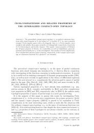
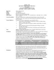
starting outline for a cause-and-effect diagram appears in Figure <strong>27</strong>.1. The main
• Describing <strong>Process</strong>es <strong>27</strong>-5<br />
FIGURE <strong>27</strong>.1<br />
Environment<br />
Material<br />
Equipment<br />
Effect<br />
An outline for a cause-and-effect diagram.<br />
To complete the diagram, group<br />
causes under these main headings in<br />
the form of branches.<br />
Personnel<br />
Methods<br />
branches organize the causes and serve as a skeleton for detailed entries. You can<br />
see why these are sometimes called “fishbone diagrams.” An example will illustrate<br />
the use of these graphs. 2<br />
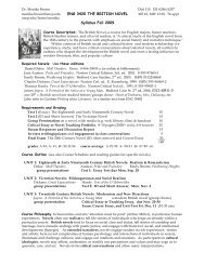
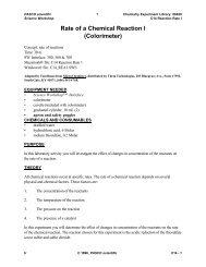
EXAMPLE <strong>27</strong>.1 Hot forging<br />
Hot forging involves heating metal to a plastic state and then shaping it by applying<br />
thousands of pounds of pressure to force the metal into a die (a kind of mold). Figure<br />
<strong>27</strong>.2 is a flowchart of a typical hot-forging process. 3<br />
A process improvement team, after making and discussing this flowchart, came to<br />
several conclusions:<br />
■ Inspecting the billets of metal received from the supplier adds no value. We<br />
should insist that the supplier be responsible for the quality of the material. The<br />
supplier should put in place good statistical process control. We can then eliminate<br />
the inspection step.<br />
■ Can we buy the metal billets already cut to rough length and ground smooth<br />
by the supplier, thus eliminating the cost of preparing the raw material ourselves?<br />
■ Heating the metal billet and forging (pressing the hot metal into the die) are the<br />
heart of the process. We should concentrate our attention here.<br />
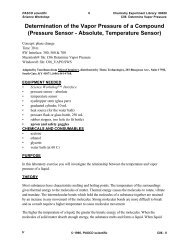
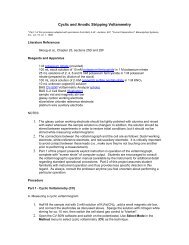
The team then prepared a cause-and-effect diagram (Figure <strong>27</strong>.3) for the heating<br />
and forging part of the process. The team members shared their specialist knowledge<br />
of the causes in their areas, resulting in a more complete picture than any one person<br />
could produce. Figure <strong>27</strong>.3 is a simplified version of the actual diagram. We have given<br />
some added detail for the “Hammer stroke” branch under “Equipment” to illustrate<br />
the next level of branches. Even this requires some knowledge of hot forging to understand.<br />
Based on detailed discussion of the diagram, the team decided what variables<br />
to measure and at what stages of the process to measure them. Producing well-chosen<br />
data is the key to improving the process. ■<br />
We will apply statistical methods to a series of measurements made on a<br />
process. Deciding what specific variables to measure is an important step in<br />
quality improvement. Often we use a “performance measure” that describes an<br />
output of a process. A company’s financial office might record the percent of<br />
errors that outside auditors find in expense account reports or the number of
<strong>27</strong>-6 <strong>CHAPTER</strong> <strong>27</strong> • <strong>Statistical</strong> <strong>Process</strong> <strong>Control</strong><br />
FIGURE <strong>27</strong>.2<br />
Flowchart of the hot-forging process<br />
in Example <strong>27</strong>.1. Use this as a model<br />
for flowcharts: decision points appear<br />
as diamonds, and other steps in the<br />
process appear as rectangles. Arrows<br />
represent flow from step to step.<br />
Receive the material<br />
Check for<br />
size and metallurgy<br />
O.K.<br />
No<br />
Scrap<br />
Yes<br />
Cut to the billet<br />
length<br />
Deburr<br />
Yes<br />
Check for<br />
size<br />
O.K.<br />
No<br />
Oversize<br />
No<br />
Scrap<br />
Yes<br />
Heat billet to the<br />
required temperature<br />
Forge to the size<br />
Flash trim<br />
and wash<br />
Shot blast<br />
Check for<br />
size and metallurgy<br />
O.K.<br />
Yes<br />
Bar code and store<br />
No<br />
Scrap<br />
data entry errors per week. The personnel department may measure the time to<br />
process employee insurance claims or the percent of job offers that are accepted.<br />
In the case of complex processes, it is wise to measure key steps within the<br />
process rather than just final outputs. The process team in Example <strong>27</strong>.1 might<br />
recommend that the temperature of the die and of the billet be measured just<br />
before forging.
• Describing <strong>Process</strong>es <strong>27</strong>-7<br />
Environment<br />
Dust in<br />
the die<br />
Humidity<br />
Temperature<br />
setup<br />
Personnel<br />
Material<br />
Billet<br />
size<br />
Air<br />
quality<br />
Handling from<br />
furnace to press<br />
Kiss blocks<br />
setup<br />
Billet<br />
metallurgy<br />
Die position<br />
and lubrication<br />
Methods<br />
Equipment<br />
Billet<br />
temperature<br />
Hammer force<br />
and stroke<br />
Billet<br />
preparation<br />
Die<br />
position<br />
Hammer stroke<br />
Loading<br />
accuracy<br />
Height<br />
Strain gauge<br />
setup<br />
Air<br />
pressure<br />
Weight<br />
Die<br />
temperature<br />
Good<br />
forged<br />
item<br />
FIGURE <strong>27</strong>.3<br />
Simplified cause-and-effect diagram of the hot-forging process in Example <strong>27</strong>.1. Good cause-andeffect<br />
diagrams require detailed knowledge of the specific process.<br />
APPLY YOUR KNOWLEDGE<br />
<strong>27</strong>.1 Describe a process. Choose a process that you know well. If you lack experience<br />
with actual business or manufacturing processes, choose a personal process<br />
such as ordering something over the Internet, paying a bill online, or recording<br />
a TV show on a DVR. Make a flowchart of the process. Make a cause-andeffect<br />
diagram that presents the factors that lead to successful completion of<br />
the process.<br />
<strong>27</strong>.2 Describe a process. Each weekday morning, you must get to work or to<br />
your first class on time. Make a flowchart of your daily process for doing this,<br />
starting when you wake. Be sure to include the time at which you plan to start<br />
each step.<br />
<strong>27</strong>.3 <strong>Process</strong> measurement. Based on your description of the process in Exercise<br />
<strong>27</strong>.1, suggest specific variables that you might measure in order to<br />
(a) assess the overall quality of the process.<br />
(b) gather information on a key step within the process.<br />
<strong>27</strong>.4 Pareto charts. Pareto charts are bar graphs with the bars ordered by height.<br />
They are often used to isolate the “vital few” categories on which we should focus<br />
our attention. Here is an example. A large medical center, financially pressed by<br />
restrictions on reimbursement by insurers and the government, looked at losses<br />
broken down by diagnosis. Government standards place cases into Diagnostic<br />
Related Groups (DRGs). For example, major joint replacements (mostly hip and<br />
knee) are DRG 209. 4 Here is what the hospital found:<br />
Pareto charts
<strong>27</strong>-8 <strong>CHAPTER</strong> <strong>27</strong> • <strong>Statistical</strong> <strong>Process</strong> <strong>Control</strong><br />
DRG<br />
Percent of losses<br />
104 5.2<br />
107 10.1<br />
109 7.7<br />
116 13.7<br />
148 6.8<br />
209 15.2<br />
403 5.6<br />
430 6.8<br />
462 9.4<br />
What percent of total losses do these 9 DRGs account for? Make a Pareto chart of<br />
losses by DRG. Which DRGs should the hospital study first when attempting to<br />
reduce its losses? DRG<br />
<strong>27</strong>.5 Pareto charts. Continue the study of the process of getting to work or class on<br />
time from Exercise <strong>27</strong>.2. If you kept good records, you could make a Pareto chart<br />
of the reasons (special causes) for late arrivals at work or class. Make a Pareto chart<br />
that you think roughly describes your own reasons for lateness. That is, list the<br />
reasons from your experience and chart your estimates of the percent of late arrivals<br />
each reason explains.<br />
<strong>27</strong>.6 Pareto charts. A large hospital was concerned about whether it was scheduling<br />
its operating rooms efficiently. Operating rooms lying idle may mean loss of potential<br />
revenue. Of particular interest was when and for how long the first operation<br />
of the day was performed. As a first step in understanding the use of its operating<br />
rooms, data were collected on what medical specialties were the first to use one of<br />
the rooms for an operation in the morning. 5 Here is what the hospital found:<br />
Specialty<br />
Percent of all operations<br />
Burns Center 3.7<br />
ENT specialist 7.6<br />
Gynecology 5.9<br />
Opthalmology 7.2<br />
Orthopedics 12.3<br />
Plastic surgery 21.1<br />
Surgery 30.6<br />
Urology 7.2<br />
What percent of total operations do these 8 specialties account for? Make a Pareto<br />
chart of percent of all operations by specialty. Which specialties should the hospital<br />
study first when attempting to understand operating-room use? OPERATIONS
• The Idea of <strong>Statistical</strong> <strong>Process</strong> <strong>Control</strong> <strong>27</strong>-9<br />
THE IDEA OF STATISTICAL PROCESS CONTROL<br />
The goal of statistical process control is to make a process stable over time<br />
and then keep it stable unless planned changes are made. You might want, for<br />
example, to keep your weight constant over time. A manufacturer of machine<br />
parts wants the critical dimensions to be the same for all parts. “Constant over<br />
time” and “the same for all” are not realistic requirements. They ignore the fact<br />
that all processes have variation. Your weight fluctuates from day to day; the critical<br />
dimension of a machined part varies a bit from item to item; the time to process a<br />
college admission application is not the same for all applications. Variation occurs<br />
in even the most precisely made product due to small changes in the raw material,<br />
the adjustment of the machine, the behavior of the operator, and even the<br />
temperature in the plant. Because variation is always present, we can’t expect to<br />
hold a variable exactly constant over time. The statistical description of stability<br />
over time requires that the pattern of variation remain stable, not that there be no<br />
variation in the variable measured.<br />
STATISTICAL CONTROL<br />
A variable that continues to be described by the same distribution when observed<br />
over time is said to be in statistical control, or simply in control.<br />
<strong>Control</strong> charts are statistical tools that monitor a process and alert us when the process<br />
has been disturbed so that it is now out of control. This is a signal to find and<br />
correct the cause of the disturbance.<br />
In the language of statistical quality control, a process that is in control has<br />
only common cause variation. Common cause variation is the inherent variability<br />
of the system, due to many small causes that are always present. When<br />
the normal functioning of the process is disturbed by some unpredictable event,<br />
special cause variation is added to the common cause variation. We hope to be<br />
able to discover what lies behind special cause variation and eliminate that cause<br />
to restore the stable functioning of the process.<br />
common cause<br />
special cause<br />
EXAMPLE <strong>27</strong>.2 Common cause, special cause<br />
Imagine yourself doing the same task repeatedly, say folding an advertising flyer, stuffing<br />
it into an envelope, and sealing the envelope. The time to complete the task will<br />
vary a bit, and it is hard to point to any one reason for the variation. Your completion<br />
time shows only common cause variation.<br />
Now the telephone rings. You answer, and though you continue folding and stuffing<br />
while talking, your completion time rises beyond the level expected from common<br />
causes alone. Answering the telephone adds special cause variation to the common<br />
cause variation that is always present. The process has been disturbed and is no longer<br />
in its normal and stable state.<br />
If you are paying temporary employees to fold and stuff advertising flyers, you avoid<br />
this special cause by not having telephones present and by asking the employees to<br />
turn off their cell phones while they are working. ■
<strong>27</strong>-10 <strong>CHAPTER</strong> <strong>27</strong> • <strong>Statistical</strong> <strong>Process</strong> <strong>Control</strong><br />
<strong>Control</strong> charts work by distinguishing the always-present common cause variation<br />
in a process from the additional variation that suggests that the process has<br />
been disturbed by a special cause. A control chart sounds an alarm when it sees<br />
too much variation. The most common application of control charts is to monitor<br />
the performance of industrial and business processes. The same methods, however,<br />
can be used to check the stability of quantities as varied as the ratings of a<br />
television show, the level of ozone in the atmosphere, and the gas mileage of your<br />
car. <strong>Control</strong> charts combine graphical and numerical descriptions of data with use<br />
of sampling distributions.<br />
APPLY YOUR KNOWLEDGE<br />
<strong>27</strong>.7 Special causes. Tayler participates in 10-kilometer races. She regularly runs 15<br />
kilometers over the same course in training. Her time varies a bit from day to day<br />
but is generally stable. Give several examples of special causes that might raise<br />
Tayler’s time on a particular day.<br />
<strong>27</strong>.8 Common causes, special causes. In Exercise <strong>27</strong>.1, you described a process<br />
that you know well. What are some sources of common cause variation in this<br />
process? What are some special causes that might at times drive the process out<br />
of control?<br />
<strong>27</strong>.9 Common causes, special causes. Each weekday morning, you must get to<br />
work or to your first class on time. The time at which you reach work or class<br />
varies from day to day, and your planning must allow for this variation. List several<br />
common causes of variation in your arrival time. Then list several special<br />
causes that might result in unusual variation leading to either early or (more<br />
likely) late arrival.<br />
chart setup<br />
process monitoring<br />
x CHARTS FOR PROCESS MONITORING<br />
When you first apply control charts to a process, the process may not be in control.<br />
Even if it is in control, you don’t yet understand its behavior. You will have<br />
to collect data from the process, establish control by uncovering and removing<br />
special causes, and then set up control charts to maintain control. We call this<br />
the chart setup stage. Later, when the process has been operating in control for<br />
some time, you understand its usual behavior and have a long run of data from the<br />
process. You keep control charts to monitor the process because a special cause<br />
could erupt at any time. We will call this process monitoring. 6<br />
Although in practice chart setup precedes process monitoring, the big ideas of<br />
control charts are more easily understood in the process-monitoring setting. We<br />
will start there, then discuss the more complex chart setup setting.<br />
Choose a quantitative variable x that is an important measure of quality. The<br />
variable might be the diameter of a part, the number of envelopes stuffed in an<br />
hour, or the time to respond to a customer call. Here are the conditions for process<br />
monitoring.
• x Charts for <strong>Process</strong> Monitoring <strong>27</strong>-11<br />
PROCESS-MONITORING CONDITIONS<br />
Measure a quantitative variable x that has a Normal distribution. The process has<br />
been operating in control for a long period, so that we know the process mean and<br />
the process standard deviation that describe the distribution of x as long as the<br />
process remains in control.<br />
In practice, we must of course estimate the process mean and standard deviation<br />
from past data on the process. Under the process-monitoring conditions, we<br />
have very many observations and the process has remained in control. The law<br />
of large numbers tells us that estimates from past data will be very close to the<br />
truth about the process. That is, at the process-monitoring stage we can act as if<br />
we know the true values of and . Note carefully that and describe<br />
the center and spread of the variable x only as long as the process remains in<br />
control. A special cause may at any time disturb the process and change<br />
the mean, the standard deviation, or both.<br />
To make control charts, begin by taking small samples from the process at<br />
regular intervals. For example, we might measure 4 or 5 consecutive parts or time<br />
the responses to 4 or 5 consecutive customer calls. There is an important idea<br />
here: the observations in a sample are so close together that we can assume that the<br />
process is stable during this short period of time. Variation within the same sample<br />
gives us a benchmark for the common cause variation in the process. The process<br />
standard deviation refers to the standard deviation within the time period spanned by<br />
one sample. If the process remains in control, the same describes the standard<br />
deviation of observations across any time period. <strong>Control</strong> charts help us decide<br />
whether this is the case.<br />
We start with the x chart based on plotting the means of the successive samples.<br />
Here is the outline:<br />
1. Take samples of size n from the process at regular intervals. Plot the means<br />
x of these samples against the order in which the samples were taken.<br />
2. We know that the sampling distribution of x under the process-monitoring<br />
conditions is Normal with mean and standard deviation s/ 1n (see text<br />
page 294). Draw a solid center line on the chart at height .<br />
3. The 99.7 part of the 68–95–99.7 rule for Normal distributions (text page<br />
77) says that, as long as the process remains in control, 99.7% of the values<br />
of x will fall between m 3s/ 1n and m 3s/ 1n. Draw dashed control<br />
limits on the chart at these heights. The control limits mark off the range of<br />
variation in sample means that we expect to see when the process remains<br />
in control.<br />
If the process remains in control and the process mean and standard deviation<br />
do not change, we will rarely observe an x outside the control limits. Such an x is<br />
therefore a signal that the process has been disturbed.<br />
x _ chart<br />
center line<br />
control limits
<strong>27</strong>-12 <strong>CHAPTER</strong> <strong>27</strong> • <strong>Statistical</strong> <strong>Process</strong> <strong>Control</strong><br />
MONITORS<br />
EXAMPLE <strong>27</strong>.3 Manufacturing computer monitors<br />
A manufacturer of computer monitors must control the tension on the mesh of<br />
fine vertical wires that lies behind the surface of the viewing screen. Too much<br />
tension will tear the mesh, and too little will allow wrinkles. Tension is measured<br />
by an electrical device with output readings in millivolts (mV). The manufacturing<br />
process has been stable with mean tension <strong>27</strong>5 mV and process standard<br />
deviation 43 mV.<br />
The mean <strong>27</strong>5 mV and the common cause variation measured by the standard<br />
deviation 43 mV describe the stable state of the process. If these values are not satisfactory—for<br />
example, if there is too much variation among the monitors—the manufacturer<br />
must make some fundamental change in the process. This might involve buying<br />
new equipment or changing the alloy used in the wires of the mesh. In fact, the common<br />
cause variation in mesh tension does not affect the performance of the monitors.<br />
We want to watch the process and maintain its current condition.<br />
The operator measures the tension on a sample of 4 monitors each hour. Table <strong>27</strong>.1<br />
gives the last 20 samples. The table also gives the mean x and the standard deviation<br />
s for each sample. The operator did not have to calculate these—modern measuring<br />
TABLE <strong>27</strong>.1 Twenty control chart samples of mesh tension<br />
(in millivolts)<br />
SAMPLE<br />
STANDARD<br />
SAMPLE TENSION MEASUREMENTS MEAN DEVIATION<br />
1 234.5 <strong>27</strong>2.3 234.5 <strong>27</strong>2.3 253.4 21.8<br />
2 311.1 305.8 238.5 286.2 285.4 33.0<br />
3 247.1 205.3 252.6 316.1 255.3 45.7<br />
4 215.4 296.8 <strong>27</strong>4.2 256.8 260.8 34.4<br />
5 3<strong>27</strong>.9 247.2 283.3 232.6 <strong>27</strong>2.7 42.5<br />
6 304.3 236.3 201.8 238.5 245.2 42.8<br />
7 268.9 <strong>27</strong>6.2 <strong>27</strong>5.6 240.2 265.2 17.0<br />
8 282.1 247.7 259.8 <strong>27</strong>2.8 265.6 15.0<br />
9 260.8 259.9 247.9 345.3 <strong>27</strong>8.5 44.9<br />
10 329.3 231.8 307.2 <strong>27</strong>3.4 285.4 42.5<br />
11 266.4 249.7 231.5 265.2 253.2 16.3<br />
12 168.8 330.9 333.6 318.3 287.9 79.7<br />
13 349.9 334.2 292.3 301.5 319.5 <strong>27</strong>.1<br />
14 235.2 283.1 245.9 263.1 256.8 21.0<br />
15 257.3 218.4 296.2 <strong>27</strong>5.2 261.8 33.0<br />
16 235.1 252.7 300.6 297.6 <strong>27</strong>1.5 32.7<br />
17 286.3 293.8 236.2 <strong>27</strong>5.3 <strong>27</strong>2.9 25.6<br />
18 328.1 <strong>27</strong>2.6 329.7 260.1 297.6 36.5<br />
19 316.4 287.4 373.0 286.0 315.7 40.7<br />
20 296.8 350.5 280.6 259.8 296.9 38.8
• x Charts for <strong>Process</strong> Monitoring <strong>27</strong>-13<br />
400<br />
350<br />
FIGURE <strong>27</strong>.4<br />
(a) Plot of the sample means versus<br />
sample number for the mesh tension<br />
data of Table <strong>27</strong>.1. (b) x chart for the<br />
mesh tension data of Table <strong>27</strong>.1. No<br />
points lie outside the control limits.<br />
Sample mean<br />
300<br />
250<br />
200<br />
150<br />
1 2 3 4 5 6 7 8 9 10 11 12 13 14 15 16 17 18 19 20<br />
Sample number<br />
(a)<br />
400<br />
350<br />
UCL<br />
Sample mean<br />
300<br />
250<br />
200<br />
LCL<br />
150<br />
1 2 3 4 5 6 7 8 9 10 11 12 13 14 15 16 17 18 19 20<br />
Sample number<br />
(b)<br />
equipment often comes equipped with software that automatically records x and s<br />
and even produces control charts. Figure <strong>27</strong>.4(a) is a plot of the sample means versus<br />
sample number. ■<br />
Figure <strong>27</strong>.4(b) is an x control chart for the 20 mesh tension samples in Table<br />
<strong>27</strong>.1. We have plotted each sample mean from the table against its sample number.<br />
For example, the mean of the first sample is 253.4 mV, and this is the value
<strong>27</strong>-14 <strong>CHAPTER</strong> <strong>27</strong> • <strong>Statistical</strong> <strong>Process</strong> <strong>Control</strong><br />
plotted for Sample 1. The center line is at <strong>27</strong>5 mV. The upper and lower<br />
control limits are<br />
s<br />
m 3<br />
2n <strong>27</strong>5 3 43<br />
<strong>27</strong>5 64.5 339.5 mV<br />
24<br />
(UCL)<br />
s<br />
m 3<br />
2n <strong>27</strong>5 3 43<br />
<strong>27</strong>5 64.5 210.5 mV<br />
24<br />
(LCL)<br />
As is common, we have labeled the control limits UCL for upper control limit<br />
and LCL for lower control limit.<br />
EXAMPLE <strong>27</strong>.4 Interpreting x charts<br />
Figure <strong>27</strong>.4(b) is a typical x chart for a process in control. The means of the 20 samples<br />
do vary, but all lie within the range of variation marked out by the control limits. We<br />
are seeing the common cause variation of a stable process.<br />
Figures <strong>27</strong>.5 and <strong>27</strong>.6 illustrate two ways in which the process can go out of control.<br />
In Figure <strong>27</strong>.5, the process was disturbed by a special cause sometime between Sample<br />
12 and Sample 13. As a result, the mean tension for Sample 13 falls above the upper<br />
control limit. It is common practice to mark all out-of-control points with an “x” to<br />
call attention to them. A search for the cause begins as soon as we see a point out of<br />
control. Investigation finds that the mounting of the tension-measuring device had<br />
slipped, resulting in readings that were too high. When the problem was corrected,<br />
Samples 14 to 20 were again in control.<br />
Figure <strong>27</strong>.6 shows the effect of a steady upward drift in the process center, starting at<br />
Sample 11. You see that some time elapses before the x for Sample 18 is out of control.<br />
<strong>Process</strong> drift results from gradual changes such as the wearing of a cutting tool or overheating.<br />
The one-point-out signal works better for detecting sudden large disturbances<br />
than for detecting slow drifts in a process. ■<br />
400<br />
350<br />
UCL<br />
x<br />
Sample mean<br />
300<br />
250<br />
FIGURE <strong>27</strong>.5<br />
This x chart is identical to that in<br />
Figure <strong>27</strong>.4(b) except that a special<br />
cause has driven x for Sample 13<br />
above the upper control limit. The<br />
out-of-control point is marked with<br />
an x.<br />
200<br />
150<br />
LCL<br />
1 2 3 4 5 6 7 8 9 10 11 12 13 14 15 16 17 18 19 20<br />
Sample number
• x Charts for <strong>Process</strong> Monitoring <strong>27</strong>-15<br />
400<br />
x<br />
x<br />
350<br />
UCL<br />
x<br />
Sample mean<br />
300<br />
250<br />
200<br />
LCL<br />
150<br />
1 2 3 4 5 6 7 8 9 10 11 12 13 14 15 16 17 18 19 20<br />
Sample number<br />
FIGURE <strong>27</strong>.6<br />
The first 10 points on this x chart are as in Figure <strong>27</strong>.4(b). The process mean drifts upward after Sample<br />
10, and the sample means x reflect this drift. The points for Samples 18, 19, and 20 are out of control.<br />
APPLY YOUR KNOWLEDGE<br />
<strong>27</strong>.10 Dry bleach. The net weight (in ounces) of boxes of dry bleach are monitored by<br />
taking samples of 4 boxes from each hour’s production. The process mean should<br />
be 16 oz. Past experience indicates that the net weight when the process in<br />
properly adjusted varies with 0.4 oz. The mean weight x for each hour’s sample<br />
is plotted on an x control chart. Calculate the center line and control limits for this<br />
chart.<br />
<strong>27</strong>.11 Tablet hardness. A pharmaceutical manufacturer forms tablets by compressing<br />
a granular material that contains the active ingredient and various fillers. The<br />
hardness of a sample from each lot of tablets is measured in order to control the<br />
compression process. The process has been operating in control with mean at<br />
the target value 11.5 kilograms (kg) and estimated standard deviation <br />
0.2 kg. Table <strong>27</strong>.2 gives three sets of data, each representing x for 20 successive<br />
samples of n 4 tablets. One set remains in control at the target value. In a<br />
second set, the process mean shifts suddenly to a new value. In a third, the<br />
process mean drifts gradually.<br />
(a) What are the center line and control limits for an x chart for this process?<br />
(b) Draw a separate x chart for each of the three data sets. Mark any points that<br />
are beyond the control limits.<br />
(c) Based on your work in (b) and the appearance of the control charts, which set<br />
of data comes from a process that is in control? In which case does the process<br />
mean shift suddenly, and at about which sample do you think that the mean<br />
changed? Finally, in which case does the mean drift gradually? HARDNESS
<strong>27</strong>-16 <strong>CHAPTER</strong> <strong>27</strong> • <strong>Statistical</strong> <strong>Process</strong> <strong>Control</strong><br />
TABLE <strong>27</strong>.2 Three sets of x _ ’s from 20 samples of size 4<br />
SAMPLE DATA SET A DATA SET B DATA SET C<br />
1 11.602 11.6<strong>27</strong> 11.495<br />
2 11.547 11.613 11.475<br />
3 11.312 11.493 11.465<br />
4 11.449 11.602 11.497<br />
5 11.401 11.360 11.573<br />
6 11.608 11.374 11.563<br />
7 11.471 11.592 11.321<br />
8 11.453 11.458 11.533<br />
9 11.446 11.552 11.486<br />
10 11.522 11.463 11.502<br />
11 11.664 11.383 11.534<br />
12 11.823 11.715 11.624<br />
13 11.629 11.485 11.629<br />
14 11.602 11.509 11.575<br />
15 11.756 11.429 11.730<br />
16 11.707 11.477 11.680<br />
17 11.612 11.570 11.729<br />
18 11.628 11.623 11.704<br />
19 11.603 11.472 12.052<br />
20 11.816 11.531 11.905<br />
s CHARTS FOR PROCESS MONITORING<br />
The x charts in Figures <strong>27</strong>.4(b), <strong>27</strong>.5, and <strong>27</strong>.6 were easy to interpret because<br />
the process standard deviation remained fixed at 43 mV. The effects of moving<br />
the process mean away from its in-control value (<strong>27</strong>5 mV) are then clear to see.<br />
We know that even the simplest description of a distribution should give both a<br />
measure of center and a measure of spread. So it is with control charts. We must<br />
monitor both the process center, using an x chart, and the process spread, using a<br />
control chart for the sample standard deviation s.<br />
The standard deviation s does not have a Normal distribution, even approximately.<br />
Under the process-monitoring conditions, the sampling distribution<br />
of s is skewed to the right. Nonetheless, control charts for any statistic are<br />
based on the “plus or minus three standard deviations” idea motivated by<br />
the 68–95–99.7 rule for Normal distributions. <strong>Control</strong> charts are intended to<br />
be practical tools that are easy to use. Standard practice in process control<br />
therefore ignores such details as the effect of non-Normal sampling distributions.<br />
Here is the general control chart setup for a sample statistic Q (short for<br />
“quality characteristic”).
• s Charts for <strong>Process</strong> Monitoring <strong>27</strong>-17<br />
THREE-SIGMA CONTROL CHARTS<br />
To make a three-sigma (3) control chart for any statistic Q:<br />
1. Take samples from the process at regular intervals and plot the values of the statistic<br />
Q against the order in which the samples were taken.<br />
2. Draw a center line on the chart at height Q , the mean of the statistic when the<br />
process is in control.<br />
3. Draw upper and lower control limits on the chart three standard deviations of Q<br />
above and below the mean. That is,<br />
UCL m Q 3s Q<br />
LCL m Q 3s Q<br />
Here Q is the standard deviation of the sampling distribution of the statistic Q<br />
when the process is in control.<br />
4. The chart produces an out-of-control signal when a plotted point lies outside the<br />
control limits.<br />
We have applied this general idea to x charts. If and are the process mean<br />
and standard deviation, the statistic x has mean m x m and standard deviation<br />
s x s/ 1n. The center line and control limits for x charts follow from these<br />
facts.<br />
What are the corresponding facts for the sample standard deviation s? Study<br />
of the sampling distribution of s for samples from a Normally distributed process<br />
characteristic gives these facts:<br />
1. The mean of s is a constant times the process standard deviation , s c 4 .<br />
2. The standard deviation of s is also a constant times the process standard deviation,<br />
s c s .<br />
The constants are called c 4 and c 5 for historical reasons. Their values depend<br />
on the size of the samples. For large samples, c 4 is close to 1. That is, the sample<br />
standard deviation s has little bias as an estimator of the process standard<br />
deviation . Because statistical process control often uses small samples, we<br />
pay attention to the value of c 4 . Following the general pattern for three-sigma<br />
control charts:<br />
1. The center line of an s chart is at c 4 .<br />
2. The control limits for an s chart are at<br />
UCL m s 3s s c 4 s 3c 5 s 1c 4 3c 5 2s<br />
LCL m s 3s s c 4 s 3c 5 s 1c 4 3c 5 2s<br />
That is, the control limits UCL and LCL are also constants times the process<br />
standard deviation. These constants are called (again for historical reasons)<br />
B 6 and B 5 . We don’t need to remember that B 6 c 4 3c 5 and B 5 c 4 3c 5 ,<br />
because tables give us the numerical values of B 6 and B 5 .
<strong>27</strong>-18 <strong>CHAPTER</strong> <strong>27</strong> • <strong>Statistical</strong> <strong>Process</strong> <strong>Control</strong><br />
x _ AND s CONTROL CHARTS FOR PROCESS MONITORING 7<br />
Take regular samples of size n from a process that has been in control with process mean <br />
and process standard deviation . The center line and control limits for an x chart are<br />
s<br />
UCL m 3<br />
2n<br />
CL m<br />
s<br />
LCL m 3<br />
2n<br />
The center line and control limits for an s chart are<br />
UCL B 6 s<br />
CL c 4 s<br />
L CL B 5 s<br />
The control chart constants c 4, B 5 , and B 6 depend on the sample size n.<br />
Table <strong>27</strong>.3 gives the values of the control chart constants c 4 , c 5 , B 5 , and B 6 for<br />
samples of sizes 2 to 10. This table makes it easy to draw s charts. The table has<br />
no B 5 entries for samples of size smaller than n 6. The lower control limit for<br />
an s chart is zero for samples of sizes 2 to 5. This is a consequence of the fact that<br />
s has a right-skewed distribution and takes only values greater than zero. Three<br />
standard deviations above the mean (UCL) lies on the long right side of the distribution.<br />
Three standard deviations below the mean (LCL) on the short left side<br />
is below zero, so we say that LCL 0.<br />
TABLE <strong>27</strong>.3 <strong>Control</strong> chart constants<br />
SAMPLE SIZE n c 4 c 5 B 5 B 6<br />
2 0.7979 0.6028 2.606<br />
3 0.8862 0.4633 2.<strong>27</strong>6<br />
4 0.9213 0.3889 2.088<br />
5 0.9400 0.3412 1.964<br />
6 0.9515 0.3076 0.029 1.874<br />
7 0.9594 0.2820 0.113 1.806<br />
8 0.9650 0.2622 0.179 1.751<br />
9 0.9693 0.2459 0.232 1.707<br />
10 0.97<strong>27</strong> 0.2321 0.<strong>27</strong>6 1.669<br />
EXAMPLE <strong>27</strong>.5 x and s charts for mesh tension<br />
Figure <strong>27</strong>.7 is the s chart for the computer monitor mesh tension data in Table <strong>27</strong>.1.<br />
The samples are of size n 4 and the process standard deviation in control is s 43<br />
mV. The center line is therefore<br />
CL c 4 s 10.921321432 39.6 mV
• s Charts for <strong>Process</strong> Monitoring <strong>27</strong>-19<br />
Sample standard deviation<br />
120<br />
100<br />
80<br />
60<br />
40<br />
20<br />
0<br />
UCL<br />
LCL<br />
1 2 3 4 5 6 7 8 9 10 11 12 13 14 15 16 17 18 19 20<br />
Sample number<br />
FIGURE <strong>27</strong>.7<br />
s chart for the mesh tension data of<br />
Table <strong>27</strong>.1. Both the s chart and the x<br />
chart (Figure <strong>27</strong>.4(b)) are in control.<br />
The control limits are<br />
UCL B 6 s 12.08821432 89.8<br />
LCL B 5 s 1021432 0<br />
Figures <strong>27</strong>.4(b) and <strong>27</strong>.7 go together: they are x and s charts for monitoring the meshtensioning<br />
process. Both charts are in control, showing only common cause variation<br />
within the bounds set by the control limits.<br />
Figures <strong>27</strong>.8 and <strong>27</strong>.9 are x and s charts for the mesh-tensioning process when a new<br />
and poorly trained operator takes over between Samples 10 and 11. The new operator<br />
400<br />
350<br />
UCL<br />
x<br />
Sample mean<br />
300<br />
250<br />
200<br />
150<br />
LCL<br />
1 2 3 4 5 6 7 8 9 10 11 12 13 14 15 16 17 18 19 20<br />
Sample number<br />
FIGURE <strong>27</strong>.8<br />
x chart for mesh tension when the<br />
process variability increases after<br />
Sample 10. The x chart does show the<br />
increased variability, but the s chart is<br />
clearer and should be read first.
<strong>27</strong>-20 <strong>CHAPTER</strong> <strong>27</strong> • <strong>Statistical</strong> <strong>Process</strong> <strong>Control</strong><br />
FIGURE <strong>27</strong>.9<br />
s chart for mesh tension when the<br />
process variability increases after<br />
Sample 10. Increased within-sample<br />
variability is clearly visible. Find and<br />
remove the s-type special cause before<br />
reading the x chart.<br />
Sample standard deviation<br />
120<br />
100<br />
80<br />
60<br />
40<br />
20<br />
UCL<br />
x<br />
x<br />
x<br />
0<br />
LCL<br />
1 2 3 4 5 6 7 8 9 10 11 12 13 14 15 16 17 18 19 20<br />
Sample number<br />
introduces added variation into the process, increasing the process standard deviation<br />
from its in-control value of 43 mV to 60 mV. The x chart in Figure <strong>27</strong>.8 shows one point<br />
out of control. Only on closer inspection do we see that the spread of the x’s increases<br />
after Sample 10. In fact, the process mean has remained unchanged at <strong>27</strong>5 mV. The<br />
apparent lack of control in the x chart is entirely due to the larger process<br />
variation. There is a lesson here: it is difficult to interpret an x chart unless s is in<br />
control. When you look at x and s charts, always start with the s chart.<br />
The s chart in Figure <strong>27</strong>.9 shows lack of control starting at Sample 11. As usual,<br />
we mark the out-of-control points with an “x” The points for Samples 13 and 15 also<br />
lie above the UCL, and the overall spread of the sample points is much greater than<br />
for the first 10 samples. In practice, the s chart would call for action after Sample 11.<br />
We would ignore the x chart until the special cause (the new operator) for the lack of<br />
control in the s chart has been found and removed by training the operator. ■<br />
Example <strong>27</strong>.5 suggests a strategy for using x and s charts in practice. First examine<br />
the s chart. Lack of control on an s chart is due to special causes that affect<br />
the observations within a sample differently. New and nonuniform raw material,<br />
a new and poorly trained operator, and mixing results from several machines or<br />
several operators are typical “s-type” special causes.<br />
Once the s chart is in control, the stable value of the process standard deviation<br />
means that the variation within samples serves as a benchmark for detecting<br />
variation in the level of the process over the longer time periods between<br />
samples. The x chart, with control limits that depend on , does this. The x chart,<br />
as we saw in Example <strong>27</strong>.5, responds to s-type causes as well as to longer-range<br />
changes in the process, so it is important to eliminate s-type special causes first.<br />
Then the x chart will alert us to, for example, a change in process level caused by<br />
new raw material that differs from that used in the past or a gradual drift in the<br />
process level caused by wear in a cutting tool.
• s Charts for <strong>Process</strong> Monitoring <strong>27</strong>-21<br />
EXAMPLE <strong>27</strong>.6 s-type and x-type special causes<br />
A large health maintenance organization (HMO) uses control charts to monitor the<br />
process of directing patient calls to the proper department or doctor’s receptionist.<br />
Each day at a random time, 5 consecutive calls are recorded electronically. The first<br />
call today is handled quickly by an experienced operator, but the next goes to a newly<br />
hired operator who must ask a supervisor for help. The sample has a large s, and lack<br />
of control signals the need to train new hires more thoroughly.<br />
The same HMO monitors the time required to receive orders from its main supplier<br />
of pharmaceutical products. After a long period in control, the x chart shows a<br />
systematic shift downward in the mean time because the supplier has changed to a<br />
more efficient delivery service. This is a desirable special cause, but it is nonetheless a<br />
systematic change in the process. The HMO will have to establish new control limits<br />
that describe the new state of the process, with smaller process mean . ■<br />
The second setting in Example <strong>27</strong>.6 reminds us that a major change in the process<br />
returns us to the chart setup stage. In the absence of deliberate changes in the process,<br />
process monitoring uses the same values of and for long periods of time. There<br />
is one important exception: careful monitoring and removal of special causes as they<br />
occur can permanently reduce the process . If the points on the s chart remain near<br />
the center line for a long period, it is wise to update the value of to the new, smaller<br />
value and compute new values of UCL and LCL for both x and s charts.<br />
APPLY YOUR KNOWLEDGE<br />
<strong>27</strong>.12 Making cappuccino. A large chain of coffee shops records a number of performance<br />
measures. Among them is the time required to complete an order for a<br />
cappuccino, measured from the time the order is placed. Suggest some plausible<br />
examples of each of the following.<br />
(a) Reasons for common cause variation in response time.<br />
(b) s-type special causes.<br />
(c) x-type special causes.<br />
<strong>27</strong>.13 Dry bleach. In Exercise <strong>27</strong>.10 (page <strong>27</strong>-15) you gave the center line and control<br />
limits for an x chart. What are the center line and control limits for an s chart for<br />
this process?<br />
<strong>27</strong>.14 Tablet hardness. Exercise <strong>27</strong>.11 concerns process control data on the hardness<br />
of tablets (measured in kilograms) for a pharmaceutical product. Table <strong>27</strong>.4 gives<br />
data for 20 new samples of size 4, with the x and s for each sample. The process has<br />
been in control with mean at the target value 11.5 kg and standard deviation<br />
0.2 kg. HARDNESS2<br />
(a) Make both x and s charts for these data based on the information given about<br />
the process.<br />
(b) At some point, the within-sample process variation increased from 0.2 kg<br />
to 0.4 kg. About where in the 20 samples did this happen? What is the<br />
effect on the s chart? On the x chart?<br />
(c) At that same point, the process mean changed from 11.5 kg to 11.7 kg.<br />
What is the effect of this change on the s chart? On the x chart?
<strong>27</strong>-22 <strong>CHAPTER</strong> <strong>27</strong> • <strong>Statistical</strong> <strong>Process</strong> <strong>Control</strong><br />
TABLE <strong>27</strong>.4 Twenty samples of size 4, with x _ and s<br />
SAMPLE HARDNESS (KILOGRAMS) x _ s<br />
1 11.432 11.350 11.582 11.184 11.387 0.1660<br />
2 11.791 11.323 11.734 11.512 11.590 0.2149<br />
3 11.373 11.807 11.651 11.651 11.620 0.1806<br />
4 11.787 11.585 11.386 11.245 11.501 0.2364<br />
5 11.633 11.212 11.568 11.469 11.470 0.1851<br />
6 11.648 11.653 11.618 11.314 11.558 0.1636<br />
7 11.456 11.<strong>27</strong>0 11.817 11.402 11.486 0.2339<br />
8 11.394 11.754 11.867 11.003 11.504 0.3905<br />
9 11.349 11.764 11.402 12.085 11.650 0.3437<br />
10 11.478 11.761 11.907 12.091 11.809 0.2588<br />
11 11.657 12.524 11.468 10.946 11.649 0.6564<br />
12 11.820 11.872 11.829 11.344 11.716 0.2492<br />
13 12.187 11.647 11.751 12.026 11.903 0.2479<br />
14 11.478 11.222 11.609 11.<strong>27</strong>1 11.395 0.1807<br />
15 11.750 11.520 11.389 11.803 11.616 0.1947<br />
16 12.137 12.056 11.255 11.497 11.736 0.4288<br />
17 12.055 11.730 11.856 11.357 11.750 0.2939<br />
18 12.107 11.624 11.7<strong>27</strong> 12.207 11.916 0.2841<br />
19 11.933 10.658 11.708 11.<strong>27</strong>8 11.394 0.5610<br />
20 12.512 12.315 11.671 11.296 11.948 0.5641<br />
Ric Ergenbright/CORBIS<br />
<strong>27</strong>.15 Dyeing yarn. The unique colors of the cashmere sweaters your firm makes result<br />
from heating undyed yarn in a kettle with a dye liquor. The pH (acidity) of the<br />
liquor is critical for regulating dye uptake and hence the final color. There are 5<br />
kettles, all of which receive dye liquor from a common source. Twice each day, the<br />
pH of the liquor in each kettle is measured, giving samples of size 5. The process<br />
has been operating in control with 4.22 and 0.1<strong>27</strong>.<br />
(a) Give the center line and control limits for the s chart.<br />
(b) Give the center line and control limits for the x chart.<br />
<strong>27</strong>.16 Mounting-hole distances. Figure <strong>27</strong>.10 reproduces a data sheet from the floor<br />
of a factory that makes electrical meters. 8 The sheet shows measurements on the<br />
distance between two mounting holes for 18 samples of size 5. The heading informs<br />
us that the measurements are in multiples of 0.0001 inch above 0.6000 inch. That<br />
is, the first measurement, 44, stands for 0.6044 inch. All the measurements end in<br />
4. Although we don’t know why this is true, it is clear that in effect the measurements<br />
were made to the nearest 0.001 inch, not to the nearest 0.0001 inch.<br />
Calculate x and s for the first two samples. The data file contains x and s for all<br />
18 samples. Based on long experience with this process, you are keeping control<br />
charts based on 43 and 12.74. Make s and x charts for the data in Figure<br />
<strong>27</strong>.10 and describe the state of the process. MOUNTINGHOLES
• Using <strong>Control</strong> Charts <strong>27</strong>-23<br />
Part name (project)<br />
Metal frame<br />
Operator<br />
Machine<br />
R-5<br />
Date 3/7<br />
3/8<br />
Time 8:30 10:30 11:45 1:30 8:15 10:15 11:45 2:00 3:00 4:00<br />
1<br />
2<br />
3<br />
4<br />
5<br />
44<br />
44<br />
44<br />
44<br />
64<br />
64<br />
44<br />
34<br />
34<br />
54<br />
34<br />
44<br />
54<br />
44<br />
54<br />
44<br />
54<br />
54<br />
34<br />
44<br />
34<br />
14<br />
84<br />
54<br />
44<br />
34<br />
64<br />
34<br />
44<br />
44<br />
54<br />
64<br />
34<br />
44<br />
34<br />
64<br />
34<br />
54<br />
44<br />
44<br />
24<br />
54<br />
44<br />
34<br />
34<br />
34<br />
44<br />
44<br />
34<br />
34<br />
Sample<br />
measurements<br />
VARIABLES CONTROL CHART (X & R)<br />
Part No.<br />
32506<br />
Chart No.<br />
1<br />
Specification limits<br />
0.6054" ± 0.0010"<br />
Gage Unit of measure Zero equals<br />
0.0001" 0.6000"<br />
Operation (process)<br />
Distance between mounting holes<br />
3/9<br />
8:30<br />
34<br />
44<br />
34<br />
64<br />
34<br />
10:00<br />
54<br />
44<br />
24<br />
54<br />
24<br />
11:45<br />
44<br />
24<br />
34<br />
34<br />
44<br />
1:30<br />
24<br />
24<br />
54<br />
44<br />
44<br />
2:30<br />
54<br />
24<br />
54<br />
44<br />
44<br />
3:30<br />
54<br />
34<br />
24<br />
44<br />
54<br />
4:30<br />
54<br />
34<br />
74<br />
44<br />
54<br />
5:30<br />
54<br />
24<br />
64<br />
34<br />
44<br />
FIGURE <strong>27</strong>.10<br />
A process control record sheet kept by<br />
operators, for Exercise <strong>27</strong>.16. This is<br />
typical of records kept by hand when<br />
measurements are not automated.<br />
We will see in the next section why<br />
such records mention x and R control<br />
charts rather than x and s charts.<br />
Average, X<br />
Range, R<br />
20<br />
30<br />
20<br />
20<br />
70<br />
30<br />
30<br />
30<br />
30<br />
10<br />
30<br />
30<br />
20<br />
30<br />
40<br />
30<br />
40<br />
40<br />
<strong>27</strong>.17 Dyeing yarn: special causes. The process described in Exercise <strong>27</strong>.15 goes out<br />
of control. Investigation finds that a new type of yarn was recently introduced. The<br />
pH in the kettles is influenced by both the dye liquor and the yarn. Moreover, on<br />
a few occasions a faulty valve on one of the kettles had allowed water to enter that<br />
kettle; as a result, the yarn in that kettle had to be discarded. Which of these special<br />
causes appears on the s chart and which on the x chart? Explain your answer.<br />
USING CONTROL CHARTS<br />
We are now familiar with the ideas that undergird all control charts and also with<br />
the details of making x and s charts. This section discusses two topics related to<br />
using control charts in practice.<br />
x _ and R charts. We have seen that it is essential to monitor both the center<br />
and the spread of a process. <strong>Control</strong> charts were originally intended to be used by<br />
factory workers with limited knowledge of statistics in the era before even calculators,<br />
let alone software, were common. In that environment, it takes too long to<br />
calculate standard deviations. The x chart for center was therefore combined with<br />
a control chart for spread based on the sample range rather than the sample standard<br />
deviation. The range R of a sample is just the difference between the largest<br />
and smallest observations. It is easy to find R without a calculator. Using R rather<br />
than s to measure the spread of samples replaces the s chart with an R chart. It<br />
also changes the x chart because the control limits for x use the estimated process<br />
spread. So x and R charts differ in the details of both charts from x and s charts.<br />
Because the range R uses only the largest and smallest observations in a sample,<br />
it is less informative than the standard deviation s calculated from all the observations.<br />
For this reason, x and s charts are now preferred to x and R charts. R<br />
charts remain common because tradition dies hard and also because it is easier<br />
for workers to understand R than s. In this short introduction, we concentrate on<br />
the principles of control charts, so we won’t give the details of constructing x and<br />
R charts. These details appear in any text on quality control. 9 If you meet a set of<br />
sample range<br />
R chart
<strong>27</strong>-24 <strong>CHAPTER</strong> <strong>27</strong> • <strong>Statistical</strong> <strong>Process</strong> <strong>Control</strong><br />
x and R charts, remember that the interpretation of these charts is just like the<br />
interpretation of x and s charts.<br />
Additional out-of-control signals. So far, we have used only the basic “one<br />
point beyond the control limits” criterion to signal that a process may have gone<br />
out of control. We would like a quick signal when the process moves out of control,<br />
but we also want to avoid “false alarms,” signals that occur just by chance<br />
when the process is really in control. The standard 3 control limits are chosen to<br />
prevent too many false alarms, because an out-of-control signal calls for an effort<br />
to find and remove a special cause. As a result, x charts are often slow to<br />
respond to a gradual drift in the process center that continues for some time<br />
before finally forcing a reading outside the control limits. We can speed the<br />
response of a control chart to lack of control—at the cost of also enduring more<br />
false alarms—by adding patterns other than “one-point-out” as signals. The most<br />
common step in this direction is to add a runs signal to the x chart.<br />
OUT-OF-CONTROL SIGNALS<br />
x and s or x and R control charts produce an out-of-control signal if:<br />
■ One-point-out: A single point lies outside the 3 control limits of either chart.<br />
■ Run: The x chart shows 9 consecutive points above the center line or 9 consecutive<br />
points below the center line. The signal occurs when we see the 9th point of the run.<br />
EXAMPLE <strong>27</strong>.7 Using the runs signal<br />
Figure <strong>27</strong>.11 reproduces the x chart from Figure <strong>27</strong>.6. The process center began a<br />
gradual upward drift at Sample 11. The chart shows the effect of the drift—the sample<br />
400<br />
x<br />
x<br />
350<br />
UCL<br />
x<br />
Sample mean<br />
300<br />
250<br />
x<br />
200<br />
LCL<br />
FIGURE <strong>27</strong>.11<br />
x chart for mesh tension data when<br />
the process center drifts upward. The<br />
“run of 9” signal gives an out-of-control<br />
warning at Sample 17.<br />
150<br />
1 2 3 4 5 6 7 8 9 10 11 12 13 14 15 16 17 18 19 20<br />
Sample number
• Setting Up <strong>Control</strong> Charts <strong>27</strong>-25<br />
means plotted on the chart move gradually upward, with some random variation. The<br />
one-point-out signal does not call for action until Sample 18 finally produces an x<br />
above the UCL. The runs signal reacts more quickly: Sample 17 is the 9th consecutive<br />
point above the center line. ■<br />
It is a mathematical fact that the runs signal responds to a gradual drift more<br />
quickly (on the average) than the one-point-out signal does. The motivation for<br />
a runs signal is that when a process is in control, the probability of a false alarm is<br />
about the same for the runs signal as for the one-point-out signal. There are many<br />
other signals that can be added to the rules for responding to x and s or x and<br />
R charts. In our enthusiasm to detect various special kinds of loss of control,<br />
it is easy to forget that adding signals always increases the frequency of false<br />
alarms. Frequent false alarms are so annoying that the people responsible<br />
for responding soon begin to ignore out-of-control signals. It is better to use only a<br />
few signals and to reserve signals other than one-point-out and runs for processes<br />
that are known to be prone to specific special causes for which there is a tailormade<br />
signal. 10<br />
APPLY YOUR KNOWLEDGE<br />
<strong>27</strong>.18 Special causes. Is each of the following examples of a special cause most likely<br />
to first result in (i) one-point-out on the s or R chart, (ii) one-point-out on the x<br />
chart, or (iii) a run on the x chart? In each case, briefly explain your reasoning.<br />
(a) The sharpness of a power saw blade deteriorates as more items are cut.<br />
(b) Buildup of dirt reduces the precision with which parts are placed for machining.<br />
(c) A new customer service representative for a Spanish-language help line is not<br />
a native speaker and has difficulty understanding customers.<br />
(d) A nurse responsible for filling out insurance claim forms grows less attentive<br />
as her shift continues.<br />
<strong>27</strong>.19 Mixtures. Here is an artificial situation that illustrates an unusual control chart<br />
pattern. Invoices are processed and paid by two clerks, one very experienced and<br />
the other newly hired. The experienced clerk processes invoices quickly. The new<br />
hire must often refer to a handbook and is much slower. Both are quite consistent,<br />
so that their times vary little from invoice to invoice. It happens that each sample<br />
of invoices comes from one of the clerks, so that some samples are from one and<br />
some from the other clerk. Sketch the x chart pattern that will result.<br />
SETTING UP CONTROL CHARTS<br />
When you first approach a process that has not been carefully studied, it is quite<br />
likely that the process is not in control. Your first goal is to discover and remove<br />
special causes and so bring the process into control. <strong>Control</strong> charts are an important<br />
tool. <strong>Control</strong> charts for process monitoring follow the process forward in time
<strong>27</strong>-26 <strong>CHAPTER</strong> <strong>27</strong> • <strong>Statistical</strong> <strong>Process</strong> <strong>Control</strong><br />
to keep it in control. <strong>Control</strong> charts at the chart setup stage, on the other hand,<br />
look back in an attempt to discover the present state of the process. An example<br />
will illustrate the method.<br />
VISCOSITY<br />
EXAMPLE <strong>27</strong>.8 Viscosity of an elastomer<br />
The viscosity of a material is its resistance to flow when under stress. Viscosity is a<br />
critical characteristic of rubber and rubber-like compounds called elastomers, which<br />
have many uses in consumer products. Viscosity is measured by placing specimens<br />
of the material above and below a slowly rotating roller, squeezing the assembly, and<br />
recording the drag on the roller. Measurements are in “Mooney units,” named after the<br />
inventor of the instrument.<br />
A specialty chemical company is beginning production of an elastomer that is<br />
supposed to have viscosity 45 5 Mooneys. Each lot of the elastomer is produced by<br />
“cooking” raw material with catalysts in a reactor vessel. Table <strong>27</strong>.5 records x and s<br />
from samples of size n 4 lots from the first 24 shifts as production begins. 11 An s chart<br />
therefore monitors variation among lots produced during the same shift. If the s chart<br />
is in control, an x chart looks for shift-to-shift variation. ■<br />
Estimating . We do not know the process mean and standard deviation .<br />
What shall we do? Sometimes we can easily adjust the center of a process by setting<br />
some control, such as the depth of a cutting tool in a machining operation<br />
or the temperature of a reactor vessel in a pharmaceutical plant. In such cases it<br />
is usual to simply take the process mean to be the target value, the depth or<br />
temperature that the design of the process specifies as correct. The x chart then<br />
helps us keep the process mean at this target value.<br />
TABLE <strong>27</strong>.5 x _ and s for 24 samples of elastomer viscosity<br />
(in Mooneys)<br />
SAMPLE x _ s SAMPLE x _ s<br />
1 49.750 2.684 13 47.875 1.118<br />
2 49.375 0.895 14 48.250 0.895<br />
3 50.250 0.895 15 47.625 0.671<br />
4 49.875 1.118 16 47.375 0.671<br />
5 47.250 0.671 17 50.250 1.566<br />
6 45.000 2.684 18 47.000 0.895<br />
7 48.375 0.671 19 47.000 0.447<br />
8 48.500 0.447 20 49.625 1.118<br />
9 48.500 0.447 21 49.875 0.447<br />
10 46.250 1.566 22 47.625 1.118<br />
11 49.000 0.895 23 49.750 0.671<br />
12 48.125 0.671 24 48.625 0.895
There is less likely to be a “correct value” for the process mean if we are<br />
monitoring response times to customer calls or data entry errors. In Example <strong>27</strong>.8,<br />
we have the target value 45 Mooneys, but there is no simple way to set viscosity<br />
at the desired level. In such cases, we want the we use in our x chart to describe<br />
the center of the process as it has actually been operating. To do this, just take the<br />
mean of all the individual measurements in the past samples. Because the samples<br />
are all the same size, this is just the mean of the sample x’s. The overall “mean of<br />
the sample means” is therefore usually called x. For the 24 samples in Table <strong>27</strong>.5,<br />
x 1<br />
24 149.750 49.375 p 48.6252<br />
1161.125<br />
24<br />
48.380<br />
Estimating . It is almost never safe to use a “target value” for the process standard<br />
deviation because it is almost never possible to directly adjust process variation.<br />
We must estimate from past data. We want to combine the sample standard deviations<br />
s from past samples rather than use the standard deviation of all the individual<br />
observations in those samples. That is, in Example <strong>27</strong>.8, we want to combine the 24<br />
sample standard deviations in Table <strong>27</strong>.5 rather than calculate the standard deviation<br />
of the 96 observations in these samples. The reason is that it is the within-sample<br />
variation that is the benchmark against which we compare the longer-term process<br />
variation. Even if the process has been in control, we want only the variation over<br />
the short time period of a single sample to influence our value for .<br />
There are several ways to estimate from the sample standard deviations. In<br />
practice, software may use a somewhat sophisticated method and then calculate<br />
the control limits for you. We use a simple method that is traditional in quality<br />
control because it goes back to the era before software. If we are basing chart<br />
setup on k past samples, we have k sample standard deviations s 1 , s 2 , . . . , s k . Just<br />
average these to get<br />
s 1 k 1s 1 s 2 p s k 2<br />
For the viscosity example, we average the s-values for the 24 samples in Table <strong>27</strong>.5:<br />
s 1 24 12.684 0.895 p 0.8952<br />
24.156<br />
24<br />
1.0065<br />
Combining the sample s-values to estimate introduces a complication: the<br />
samples used in process control are often small (size n 4 in the viscosity example),<br />
so s has some bias as an estimator of . Recall that s c 4 . The mean s inherits this<br />
bias: its mean is also not but c 4 . The proper estimate of corrects this bias. It is<br />
• Setting Up <strong>Control</strong> Charts <strong>27</strong>-<strong>27</strong><br />
ŝ s<br />
c 4
<strong>27</strong>-28 <strong>CHAPTER</strong> <strong>27</strong> • <strong>Statistical</strong> <strong>Process</strong> <strong>Control</strong><br />
We get control limits from past data by using the estimates x and ŝ in place of the<br />
and used in charts at the process-monitoring stage. Here are the results. 12<br />
x _ AND s CONTROL CHARTS USING PAST DATA<br />
Take regular samples of size n from a process. Estimate the process mean and the<br />
process standard deviation from past samples by<br />
mˆ x<br />
ŝ s<br />
c 4<br />
(or use a target value)<br />
The center line and control limits for an x chart are<br />
ŝ<br />
UCL mˆ 3<br />
1n<br />
CL mˆ<br />
ŝ<br />
LCL mˆ 3<br />
1n<br />
The center line and control limits for an s chart are<br />
UCL B 6 ŝ<br />
CL c 4 ŝ s<br />
LCL B 5 ŝ<br />
If the process was not in control when the samples were taken, these should be regarded<br />
as trial control limits.<br />
We are now ready to outline the chart setup procedure for elastomer viscosity.<br />
Step 1. As usual, we look first at an s chart. For chart setup, control limits are<br />
based on the same past data that we will plot on the chart. Calculate from Table<br />
<strong>27</strong>.5 that<br />
s 1.0065<br />
ŝ s<br />
c 4<br />
1.0065<br />
0.9213 1.0925<br />
The center line and control limits for an s chart based on past data are<br />
UCL B 6 ŝ 12.088211.09252 2.281<br />
CL s 1.0065<br />
LCL B 5 ŝ 10211.09252 0<br />
Figure <strong>27</strong>.12 is the s chart. The points for Shifts 1 and 6 lie above the UCL. Both<br />
are near the beginning of production. Investigation finds that the reactor operator<br />
made an error on one lot in each of these samples. The error changed the viscosity<br />
of that lot and increased s for that one sample. The error will not be repeated now<br />
that the operators have gained experience. That is, this special cause has already<br />
been removed.
• Setting Up <strong>Control</strong> Charts <strong>27</strong>-29<br />
Standard deviation<br />
4.0<br />
3.5<br />
3.0<br />
x<br />
2.5 UCL<br />
2.0<br />
1.5<br />
1.0<br />
0.5<br />
x<br />
FIGURE <strong>27</strong>.12<br />
s chart based on past data for the viscosity<br />
data of Table <strong>27</strong>.5. The control<br />
limits are based on the same s-values<br />
that are plotted on the chart. Points<br />
1 and 6 are out of control.<br />
0.0<br />
2 4 6 8 10 12 14 16 18 20 22 24<br />
Sample number<br />
Step 2. Remove the two values of s that were out of control. This is proper<br />
because the special cause responsible for these readings is no longer present. Recalculate<br />
from the remaining 22 shifts that s 0.854 and ŝ 0.854/0.9213 0.9<strong>27</strong>.<br />
Make a new s chart with<br />
UCL B 6 ŝ 12.088210.9<strong>27</strong>2 1.936<br />
CL s 0.854<br />
LCL B 5 ŝ 10210.9<strong>27</strong>2 0<br />
We don’t show the chart, but you can see from Table <strong>27</strong>.5 that none of the<br />
remaining s-values lies above the new, lower, UCL; the largest remaining s is<br />
1.566. If additional points were now out of control, we would repeat the process<br />
of finding and eliminating s-type causes until the s chart for the remaining shifts<br />
was in control. In practice, of course, this is often a challenging task.<br />
Step 3. Once s-type causes have been eliminated, make an x chart using only<br />
the samples that remain after dropping those that had out-of-control s-values.<br />
For the 22 remaining samples, we know that ŝ 0.9<strong>27</strong> and we calculate that<br />
x 48.4716. The center line and control limits for the x chart are<br />
ŝ<br />
UCL x 3<br />
1n 48.4716 3 0.9<strong>27</strong><br />
14 49.862<br />
CL x 48.4716<br />
ŝ<br />
LCL x 3<br />
1n 48.4716 3 0.9<strong>27</strong><br />
14 47.081<br />
Figure <strong>27</strong>.13 is the x chart. Shifts 1 and 6 have been dropped. Seven of the 22<br />
points are beyond the 3 limits, four high and three low. Although within-shift
<strong>27</strong>-30 <strong>CHAPTER</strong> <strong>27</strong> • <strong>Statistical</strong> <strong>Process</strong> <strong>Control</strong><br />
FIGURE <strong>27</strong>.13<br />
x chart based on past data for the viscosity<br />
data of Table <strong>27</strong>.5. The samples<br />
for Shifts 1 and 6 have been removed<br />
because s-type special causes active in<br />
those samples are no longer active.<br />
The x chart shows poor control.<br />
Sample mean<br />
54<br />
52<br />
50<br />
48<br />
46<br />
UCL x x<br />
LCL<br />
x<br />
x<br />
xx<br />
x<br />
44<br />
2 4 6 8 10 12 14 16 18 20 22 24<br />
Sample number<br />
variation is now stable, there is excessive variation from shift to shift. To find the<br />
cause, we must understand the details of the process, but knowing that the special<br />
cause or causes operate between shifts is a big help. If the reactor is set up anew<br />
at the beginning of each shift, that’s one place to look more closely.<br />
Step 4. Once the x and s charts are both in control (looking backward), use<br />
the estimates mˆ and ŝ from the points in control to set tentative control limits<br />
to monitor the process going forward. If it remains in control, we can update the<br />
charts and move to the process-monitoring stage.<br />
APPLY YOUR KNOWLEDGE<br />
<strong>27</strong>.20 From setup to monitoring. Suppose that when the chart setup project of<br />
Example <strong>27</strong>.8 is complete, the points remaining after removing special causes have<br />
x 48.7 and s 0.92. What are the center line and control limits for the x and s<br />
charts you would use to monitor the process going forward?<br />
<strong>27</strong>.21 Estimating process parameters. The x and s control charts for the meshtensioning<br />
example (Figures <strong>27</strong>.4(b) (page <strong>27</strong>-13) and <strong>27</strong>.7 (page <strong>27</strong>-19)) were<br />
based on <strong>27</strong>5 mV and 43 mV. Table <strong>27</strong>.1 (page <strong>27</strong>-12) gives the 20 most<br />
recent samples from this process.<br />
(a) Estimate the process and based on these 20 samples.<br />
(b) Your calculations suggest that the process may now be less than 43 mV.<br />
Explain why the s chart in Figure <strong>27</strong>.7 (page <strong>27</strong>-19) suggests the same conclusion.<br />
(If this pattern continues, we would eventually update the value of <br />
used for control limits.) MONITORS<br />
<strong>27</strong>.22 Hospital losses. Table <strong>27</strong>.6 gives data on the losses (in dollars) incurred by a<br />
hospital in treating major joint replacement (DRG 209) patients. 13 The hospital
• Setting Up <strong>Control</strong> Charts <strong>27</strong>-31<br />
TABLE <strong>27</strong>.6 Hospital losses (dollars) for 15 samples of DRG 209 patients<br />
SAMPLE<br />
STANDARD<br />
SAMPLE LOSS MEAN DEVIATION<br />
1 6835 5843 6019 6731 6362 5696 7193 6206 6360.6 521.7<br />
2 6452 6764 7083 7352 5239 6911 7479 5549 6603.6 817.1<br />
3 7205 6374 6198 6170 6482 4763 7125 6241 6319.8 749.1<br />
4 6021 6347 7210 6384 6807 5711 7952 6023 6556.9 736.5<br />
5 7000 6495 6893 61<strong>27</strong> 7417 7044 6159 6091 6653.2 503.7<br />
6 7783 6224 5051 7288 6584 7521 6146 5129 6465.8 1034.3<br />
7 8794 6<strong>27</strong>9 6877 5807 6076 6392 7429 5220 6609.2 1104.0<br />
8 47<strong>27</strong> 8117 6586 6225 6150 7386 5674 6740 6450.6 1033.0<br />
9 5408 7452 6686 6428 6425 7380 5789 6264 6479.0 704.7<br />
10 5598 7489 6186 5837 6769 5471 5658 6393 6175.1 690.5<br />
11 6559 5855 4928 5897 7532 5663 4746 7879 6132.4 1128.6<br />
12 6824 7320 5331 6204 60<strong>27</strong> 5987 6033 6177 6237.9 596.6<br />
13 6503 8213 5417 6360 6711 6907 6625 7888 6828.0 879.8<br />
14 5622 6321 6325 6634 5075 6209 4832 6386 5925.5 667.8<br />
15 6269 6756 7653 6065 5835 7337 6615 8181 6838.9 819.5<br />
has taken from its records a random sample of 8 such patients each month for<br />
15 months. DRG2<br />
(a) Make an s control chart using center lines and limits calculated from these<br />
past data. There are no points out of control.<br />
(b) Because the s chart is in control, base the x chart on all 15 samples. Make this<br />
chart. Is it also in control?<br />
<strong>27</strong>.23 A cutting operation. A machine tool in your plant is cutting an outside diameter.<br />
A sample of 4 pieces is taken near the end of each hour of production. Table <strong>27</strong>.7<br />
TABLE <strong>27</strong>.7 x _ and s for 21 samples of outside diameter<br />
SAMPLE x _ s SAMPLE x _ s<br />
1 0.14 0.48 12 0.55 0.10<br />
2 0.09 0.26 13 0.50 0.25<br />
3 0.17 0.24 14 0.37 0.45<br />
4 0.08 0.38 15 0.69 0.21<br />
5 0.17 0.50 16 0.47 0.34<br />
6 0.36 0.26 17 0.56 0.42<br />
7 0.30 0.39 18 0.78 0.08<br />
8 0.19 0.31 19 0.75 0.32<br />
9 0.48 0.13 20 0.49 0.23<br />
10 0.29 0.13 21 0.79 0.12<br />
11 0.48 0.25
<strong>27</strong>-32 <strong>CHAPTER</strong> <strong>27</strong> • <strong>Statistical</strong> <strong>Process</strong> <strong>Control</strong><br />
gives x and s for the first 21 samples, coded in units of 0.0001 inch from the center<br />
of the specifications. The specifications allow a range of 0.0002 inch about the<br />
center (a range of 2 to 2 as coded).<br />
(a) Make an s chart based on past data and comment on control of short-term<br />
process variation.<br />
(b) Because the data are coded about the center of the specs, we have a given<br />
target 0 (as coded) for the process mean. Make an x chart and comment<br />
on control of long-term process variation. What special x-type cause probably<br />
explains the lack of control of x? CUTTING<br />
<strong>27</strong>.24 The Boston Marathon. The Boston Marathon has been run each year since<br />
1897. Winning times were highly variable in the early years, but control improved<br />
as the best runners became more professional. A clear downward trend continued<br />
until the 1980s. Rick plans to make a control chart for the winning times from<br />
1950 to the present. The first few times are 153, 148, 152, 139, 141, and 138 minutes.<br />
Calculation from the winning times from 1950 to 2011 gives<br />
x 134.032 minutes and s 6.462 minutes<br />
Rick draws a center line at x and control limits at x 3s for a plot of individual<br />
winning times. Explain carefully why these control limits are too wide to effectively<br />
signal unusually fast or slow times.<br />
COMMENTS ON STATISTICAL CONTROL<br />
Having seen how x and s (or x and R) charts work, we can turn to some important<br />
comments and cautions about statistical control in practice.<br />
Focus on the process rather than on the products. This is a fundamental<br />
idea in statistical process control. We might attempt to attain high quality by careful<br />
inspection of the finished product, measuring every completed forging and reviewing<br />
every outgoing invoice and expense account payment. Inspection of finished<br />
products can ensure good quality, but it is expensive. Perhaps more important, final<br />
inspection comes too late: when something goes wrong early in a process, much bad<br />
product may be produced before final inspection discovers the problem. This adds<br />
to the expense, because the bad product must then be scrapped or reworked.<br />
The small samples that are the basis of control charts are intended to monitor the<br />
process at key points, not to ensure the quality of the particular items in the samples.<br />
If the process is kept in control, we know what to expect in the finished product.<br />
We want to do it right the first time, not inspect and fix finished product.<br />
rational subgroup<br />
Rational subgroups. The interpretation of control charts depends on the distinction<br />
between x-type special causes and s-type special causes. This distinction in<br />
turn depends on how we choose the samples from which we calculate s (or R). We<br />
want the variation within a sample to reflect only the item-to-item chance variation<br />
that (when in control) results from many small common causes. Walter Shewhart,<br />
the founder of statistical process control, used the term rational subgroup to emphasize<br />
that we should think about the process when deciding how to choose samples.
• Comments on <strong>Statistical</strong> <strong>Control</strong> <strong>27</strong>-33<br />
EXAMPLE <strong>27</strong>.9 Random sampling versus rational subgroups<br />
A pharmaceutical manufacturer forms tablets by compressing a granular material that<br />
contains the active ingredient and various fillers. To monitor the compression process,<br />
we will measure the hardness of a sample from each 10 minutes’ production of tablets.<br />
Should we choose a random sample of tablets from the several thousand produced in<br />
a 10-minute period?<br />
A random sample would contain tablets spread across the entire 10 minutes. It fairly<br />
represents the 10-minute period, but that isn’t what we want for process control. If the<br />
setting of the press drifts or a new lot of filler arrives during the 10 minutes, the spread<br />
of the sample will be increased. That is, a random sample contains both the short-term<br />
variation among tablets produced in quick succession and the longer-term variation<br />
among tablets produced minutes apart. We prefer to measure a rational subgroup of<br />
5 consecutive tablets every 10 minutes. We expect the process to be stable during this<br />
very short time period, so that variation within the subgroups is a benchmark against<br />
which we can see special cause variation. ■<br />
Samples of consecutive items are rational subgroups when we are monitoring<br />
the output of a single activity that does the same thing over and over again.<br />
Several consecutive items is the most common type of sample for process control.<br />
There is no formula for choosing samples that are rational subgroups. You must<br />
think about causes of variation in your process and decide which you are willing<br />
to think of as common causes that you will not try to eliminate. Rational subgroups<br />
are samples chosen to express variation due to these causes and no others.<br />
Because the choice requires detailed process knowledge, we will usually accept<br />
samples of consecutive items as being rational subgroups.<br />
Why statistical control is desirable. To repeat, if the process is kept in control,<br />
we know what to expect in the finished product. The process mean and<br />
standard deviation remain stable over time, so (assuming Normal variation)<br />
the 99.7 part of the 68–95–99.7 rule tells us that almost all measurements on<br />
individual products will lie in the range 3. These are sometimes called the<br />
natural tolerances for the product. Be careful to distinguish 3, the<br />
range we expect for individual measurements, from the x chart control limits<br />
m 3s/ 1n, which mark off the expected range of sample means.<br />
natural tolerances<br />
EXAMPLE <strong>27</strong>.10 Natural tolerances for mesh tension<br />
The process of setting the mesh tension on computer monitors has been operating in<br />
control. The x and s charts were based on <strong>27</strong>5 mV and 43 mV. The s chart<br />
in Figure <strong>27</strong>.7 and your calculation in Exercise <strong>27</strong>.21 suggest that the process is now<br />
less than 43 mV. We may prefer to calculate the natural tolerances from the recent data<br />
on 20 samples (80 monitors) in Table <strong>27</strong>.1 (page <strong>27</strong>-12). The estimate of the mean is<br />
x <strong>27</strong>5.065, very close to the target value.<br />
Now a subtle point arises. The estimate ŝ s/c 4 used for past-data control charts is<br />
based entirely on variation within the samples. That’s what we want for control charts,<br />
because within-sample variation is likely to be “pure common cause” variation. Even<br />
when the process is in control, there is some additional variation from sample to
<strong>27</strong>-34 <strong>CHAPTER</strong> <strong>27</strong> • <strong>Statistical</strong> <strong>Process</strong> <strong>Control</strong><br />
sample, just by chance. So the variation in the process output will be greater than the<br />
variation within samples. To estimate the natural tolerances, we should estimate from all<br />
80 individual monitors rather than by averaging the 20 within-sample standard deviations.<br />
The standard deviation for all 80 mesh tensions is<br />
s 38.38<br />
(For a sample of size 80, c 4 is very close to 1, so we can ignore it.)<br />
We are therefore confident that almost all individual monitors will have mesh tension<br />
x 3s <strong>27</strong>5.065 132138.382 <strong>27</strong>5 115<br />
We expect mesh tension measurements to vary between 160 and 390 mV. You see that<br />
the spread of individual measurements is wider than the spread of sample means used<br />
for the control limits of the x chart. ■<br />
The natural tolerances in Example <strong>27</strong>.10 depend on the fact that the mesh<br />
tensions of individual monitors follow a Normal distribution. We know that the<br />
process was in control when the 80 measurements in Table <strong>27</strong>.1 were made, so we<br />
can graph them to assess Normality.<br />
APPLY YOUR KNOWLEDGE<br />
<strong>27</strong>.25 No incoming inspection. The computer makers who buy monitors require that<br />
the monitor manufacturer practice statistical process control and submit control<br />
charts for verification. This allows the computer makers to eliminate inspection of<br />
monitors as they arrive, a considerable cost saving. Explain carefully why incoming<br />
inspection can safely be eliminated.<br />
<strong>27</strong>.26 Natural tolerances. Table <strong>27</strong>.6 (page <strong>27</strong>-31) gives data on hospital losses for<br />
samples of DRG 209 patients. The distribution of losses has been stable over time.<br />
What are the natural tolerances within which you expect losses on nearly all such<br />
patients to fall? DRG2<br />
<strong>27</strong>.<strong>27</strong> Normality? Do the losses on the 120 individual patients in Table <strong>27</strong>.6 appear to<br />
come from a single Normal distribution? Make a graph and discuss what it shows. Are<br />
the natural tolerances you found in the previous exercise trustworthy? DRG2<br />
DON’T CONFUSE CONTROL WITH CAPABILITY!<br />
A process in control is stable over time. We know how much variation the finished<br />
product will show. <strong>Control</strong> charts are, so to speak, the voice of the process<br />
telling us what state it is in. There is no guarantee that a process in control<br />
produces products of satisfactory quality. “Satisfactory quality” is measured<br />
by comparing the product to some standard outside the process, set by<br />
technical specifications, customer expectations, or the goals of the organization.<br />
These external standards are unrelated to the internal state of the process, which<br />
is all that statistical control pays attention to.
• Don’t Confuse <strong>Control</strong> with Capability! <strong>27</strong>-35<br />
CAPABILITY<br />
Capability refers to the ability of a process to meet or exceed the requirements<br />
placed on it.<br />
Capability has nothing to do with control—except for the very important<br />
point that if a process is not in control, it is hard to tell if it is capable or not.<br />
EXAMPLE <strong>27</strong>.11 Capability<br />
The primary customer for our monitors is a large maker of computers. The customer<br />
informed us that adequate image quality requires that the mesh tension lie between 100<br />
and 400 mV. Because the mesh-tensioning process is in control, we know (Example<br />
<strong>27</strong>.10) that almost all monitors will have mesh tension between 160 and 390 mV. The<br />
process is capable of meeting the customer’s requirement.<br />
Figure <strong>27</strong>.14 compares the distribution of mesh tension for individual monitors with<br />
the customer’s specifications. The distribution of tension is approximately Normal, and<br />
we estimate its mean to be very close to <strong>27</strong>5 mV and the standard deviation to be about<br />
38.4 mV. The distribution is safely within the specifications.<br />
Times change, however. As computer buyers demand better screen quality, the<br />
computer maker restudies the effect of mesh tension and decides to require that<br />
tension lie between 150 and 350 mV. These new specification limits also appear<br />
in Figure <strong>27</strong>.14. The process is not capable of meeting the new requirements. The<br />
process remains in control. The change in its capability is entirely due to a change<br />
in external requirements. ■<br />
New<br />
specifications<br />
Old<br />
specifications<br />
100 150 <strong>27</strong>5 350<br />
Mesh tension<br />
400<br />
FIGURE <strong>27</strong>.14<br />
Comparison of the distribution of mesh tension (Normal curve) with original and tightened specifications,<br />
for Example <strong>27</strong>.11. The process in its current state is not capable of meeting the new<br />
specifications.
<strong>27</strong>-36 <strong>CHAPTER</strong> <strong>27</strong> • <strong>Statistical</strong> <strong>Process</strong> <strong>Control</strong><br />
Because the mesh-tensioning process is in control, we know that it is not<br />
capable of meeting the new specifications. That’s an advantage of control, but<br />
the fact remains that control does not guarantee capability. If a process<br />
that is in control does not have adequate capability, fundamental changes in the<br />
process are needed. The process is doing as well as it can and displays only<br />
the chance variation that is natural to its present state. Better training for workers,<br />
new equipment, or more uniform material may improve capability, depending<br />
on the findings of a careful investigation.<br />
APPLY YOUR KNOWLEDGE<br />
<strong>27</strong>.28 Describing capability. If the mesh tension of individual monitors follows a Normal<br />
distribution, we can describe capability by giving the percent of monitors that<br />
meet specifications. The old specifications for mesh tension are 100 to 400 mV.<br />
The new specifications are 150 to 350 mV. Because the process is in control, we<br />
can estimate that tension has mean <strong>27</strong>5 mV and standard deviation 38.4 mV.<br />
(a) What percent of monitors meet the old specifications?<br />
(b) What percent meet the new specifications?<br />
<strong>27</strong>.29 Improving capability. The center of the specifications for mesh tension in the<br />
previous exercise is 250 mV, but the center of our process is <strong>27</strong>5 mV. We can<br />
improve capability by adjusting the process to have center 250 mV. This is an easy<br />
adjustment that does not change the process variation. What percent of monitors<br />
now meet the new specifications?<br />
<strong>27</strong>.30 Mounting-hole distances. Figure <strong>27</strong>.10 (page <strong>27</strong>-23) displays a record sheet for<br />
18 samples of distances between mounting holes in an electrical meter. The data<br />
file adds x and s for each sample. In Exercise <strong>27</strong>.16, you found that Sample 5 was<br />
out of control on the process-monitoring s chart. The special cause responsible was<br />
found and removed. Based on the 17 samples that were in control, what are the<br />
natural tolerances for the distance between the holes? MOUNTING HOLES<br />
<strong>27</strong>.31 Mounting-hole distances, continued. The record sheet in Figure <strong>27</strong>.10 gives<br />
the specifications as 0.6054 0.0010 inch. That’s 54 10 as the data are coded on<br />
the record sheet. Assuming that the distance varies Normally from meter to meter,<br />
about what percent of meters meet the specifications?<br />
CONTROL CHARTS FOR SAMPLE PROPORTIONS<br />
We have considered control charts for just one kind of data: measurements of a<br />
quantitative variable in some meaningful scale of units. We describe the distribution<br />
of measurements by its center and spread and use x and s or x and R charts for<br />
process control. There are control charts for other statistics that are appropriate<br />
for other kinds of data. The most common of these is the p chart for use when the<br />
data are proportions.
• <strong>Control</strong> Limits for p Charts <strong>27</strong>-37<br />
p CHART<br />
A p chart is a control chart based on plotting sample proportions pˆ from regular<br />
samples from a process against the order in which the samples were taken.<br />
EXAMPLE <strong>27</strong>.12 p chart settings<br />
Here are two examples of the usefulness of p charts:<br />
■ Measure two dimensions of a manufactured part and also grade its surface finish by<br />
eye. The part conforms if both dimensions lie within their specifications and the<br />
finish is judged acceptable. Otherwise, it is nonconforming. Plot the proportion of<br />
nonconforming parts in samples of parts from each shift.<br />
■ An urban school system records the percent of its eighth-grade students who are<br />
absent three or more days each month. Because students with high absenteeism in<br />
eighth grade often fail to complete high school, the school system has launched<br />
programs to reduce absenteeism. These programs include calls to parents of absent<br />
students, public-service messages to change community expectations, and measures<br />
to ensure that the schools are safe and attractive. A p chart will show if the programs<br />
are having an effect. ■<br />
The manufacturing example illustrates an advantage of p charts: they can<br />
combine several specifications in a single chart. Nonetheless, p charts have been<br />
rendered outdated in many manufacturing applications by improvements in typical<br />
levels of quality. For example, Delphi, the largest North American auto electronics<br />
manufacturer, says that it reduced its proportion of problem parts from 200 per million<br />
in 1997 to 20 per million in 2001. 14 At either of these levels, even large samples<br />
of parts will rarely contain any bad parts. The sample proportions will almost all be<br />
0, so that plotting them is uninformative. It is better to choose important measured<br />
characteristics—voltage at a critical circuit point, for example—and keep x and s<br />
charts. Even if the voltage is satisfactory, quality can be improved by moving it yet<br />
closer to the exact voltage specified in the design of the part.<br />
The school absenteeism example is a management application of p charts.<br />
More than 20% of all American eighth-graders miss three or more days of school<br />
per month, and this proportion is higher in large cities. A p chart will be useful.<br />
Proportions of “things going wrong” are often higher in business processes than in<br />
manufacturing, so that p charts are an important tool in business.<br />
CONTROL LIMITS FOR p CHARTS<br />
We studied the sampling distribution of a sample proportion pˆ in Chapter 20. The<br />
center line and control limits for a 3 control chart follow directly from the facts<br />
stated there, in the box on text page 494. We ought to call such charts “pˆ charts”<br />
because they plot sample proportions. Unfortunately, they have always been called<br />
p charts in quality control circles. We will keep the traditional name but also keep<br />
our usual notation: p is a process proportion and pˆ is a sample proportion.
<strong>27</strong>-38 <strong>CHAPTER</strong> <strong>27</strong> • <strong>Statistical</strong> <strong>Process</strong> <strong>Control</strong><br />
p CHART USING PAST DATA<br />
Take regular samples from a process that has been in control. Estimate the process<br />
proportion p of “successes” by<br />
total number of successes in past samples<br />
p <br />
total number of individuals in these samples<br />
The center line and control limits for a p chart for future samples of size n are<br />
p 11 p2<br />
UCL p 3<br />
B n<br />
CL p<br />
p 11 p2<br />
LCL p 3<br />
B n<br />
Common out-of-control signals are one sample proportion pˆ outside the control<br />
limits or a run of 9 sample proportions on the same side of the center line.<br />
If we have k past samples of the same size n, then p is just the average of<br />
the k sample proportions. In some settings, you may meet samples of unequal<br />
size—differing numbers of students enrolled in a month or differing numbers of<br />
parts inspected in a shift. The average p estimates the process proportion p even<br />
when the sample sizes vary. Note that the control limits use the actual size n of<br />
a sample.<br />
ABSENTEEISM<br />
EXAMPLE <strong>27</strong>.13 Reducing absenteeism<br />
Unscheduled absences by clerical and production workers are an important cost in<br />
many companies. You have been asked to improve absenteeism in a production facility<br />
where 12% of the workers are now absent on a typical day.<br />
Start with data: the Pareto chart in Figure <strong>27</strong>.15 shows that there are major differences<br />
among supervisors in the absenteeism rate of their workers. You retrain all the<br />
supervisors in human relations skills, using B, E, and H as discussion leaders. In addition,<br />
a trainer works individually with supervisors I and D. You also improve lighting<br />
and other work conditions.<br />
Are your actions effective? You hope to see a reduction in absenteeism. To view<br />
progress (or lack of progress), you will keep a p chart of the proportion of absentees.<br />
The plant has 987 production workers. For simplicity, you just record the number who<br />
are absent from work each day. Only unscheduled absences count, not planned time<br />
off such as vacations. Each day you will plot<br />
pˆ <br />
number of workers absent<br />
987<br />
You first look back at data for the past three months. There were 64 workdays in these<br />
months. The total of workdays available for the workers was<br />
164219872 63,168 person-days
• <strong>Control</strong> Limits for p Charts <strong>27</strong>-39<br />
Average percent of workers absent<br />
25<br />
20<br />
15<br />
10<br />
5<br />
FIGURE <strong>27</strong>.15<br />
Pareto chart of the average absenteeism<br />
rate for workers reporting to each<br />
of 12 supervisors, for Example <strong>27</strong>.13.<br />
0<br />
I D A L F G K C J B E H<br />
Supervisor<br />
Absences among all workers totaled 7580 person-days. The average daily proportion<br />
absent was therefore<br />
total days absent<br />
p <br />
total days available for work<br />
7580<br />
<br />
63,168 0.120<br />
The daily rate has been in control at this level.<br />
These past data allow you to set up a p chart to monitor future proportions absent:<br />
p 11 p 2<br />
10.120210.8802<br />
UCL p 3<br />
0.120 3<br />
B n<br />
B 987<br />
0.120 0.031 0.151<br />
CL p 0.120<br />
p 11 p 2<br />
LCL p 3<br />
B n<br />
0.120 0.031 0.089<br />
10.120210.8802<br />
0.120 3<br />
B 987<br />
Table <strong>27</strong>.8 gives the data for the next four weeks. Figure <strong>27</strong>.16 is the p chart. ■<br />
Figure <strong>27</strong>.16 shows a clear downward trend in the daily proportion of workers<br />
who are absent. Days 13 and 19 lie below LCL, and a run of 9 days below the center<br />
line is achieved at Day 15 and continues. The points marked “x” are therefore<br />
all out of control. It appears that a special cause (the various actions you took)<br />
has reduced the absenteeism rate from around 12% to around 10%. The data for<br />
the last two weeks suggest that the rate has stabilized at this level. You will update
<strong>27</strong>-40 <strong>CHAPTER</strong> <strong>27</strong> • <strong>Statistical</strong> <strong>Process</strong> <strong>Control</strong><br />
TABLE <strong>27</strong>.8 Proportions of workers absent during four weeks<br />
M T W Th F M T W Th F<br />
Workers absent 129 121 117 109 122 119 103 103 89 105<br />
Proportion pˆ 0.131 0.123 0.119 0.110 0.124 0.121 0.104 0.104 0.090 0.106<br />
M T W Th F M T W Th F<br />
Workers absent 99 92 83 92 92 115 101 106 83 98<br />
Proportion pˆ 0.100 0.093 0.084 0.093 0.093 0.117 0.102 0.107 0.084 0.099<br />
the chart based on the new data. If the rate does not decline further (or even rises<br />
again as the effect of your actions wears off), you will consider further changes.<br />
Example <strong>27</strong>.13 is a bit oversimplified. The number of workers available did<br />
not remain fixed at 987 each day. Hirings, resignations, and planned vacations<br />
change the number a bit from day to day. The control limits for a day’s pˆ depend<br />
on n, the number of workers that day. If n varies, the control limits will move in<br />
and out from day to day. Software will do the extra arithmetic needed for a different<br />
n each day, but as long as the count of workers remains close to 987, the<br />
greater detail will not change your conclusion.<br />
A single p chart for all workers is not the only, or even the best, choice in this<br />
setting. Because of the important role of supervisors in absenteeism, it would be<br />
wise to also keep separate p charts for the workers under each supervisor. These<br />
charts may show that you must reassign some supervisors.<br />
0.18<br />
0.16<br />
UCL<br />
Proportion absent<br />
0.14<br />
0.12<br />
0.10<br />
LCL<br />
x<br />
x<br />
x<br />
x<br />
x<br />
0.08<br />
x<br />
x<br />
0.06<br />
1 2 3 4 5 6 7 8 9 10 11 12 13 14 15 16 17 18 19 20<br />
Day<br />
FIGURE <strong>27</strong>.16<br />
p chart for daily proportion of workers absent over a four-week period, for Example <strong>27</strong>.13. The<br />
lack of control shows an improvement (decrease) in absenteeism. Update the chart to continue<br />
monitoring the process.
• Apply Your Knowledge <strong>27</strong>-41<br />
APPLY YOUR KNOWLEDGE<br />
<strong>27</strong>.32 Setting up a p chart. After inspecting Figure <strong>27</strong>.16, you decide to monitor the<br />
next four weeks’ absenteeism rates using a center line and control limits calculated<br />
from the last two weeks of data recorded in Table <strong>27</strong>.8. Find p for these 10 days<br />
and give the new values of CL, LCL, and UCL. (Until you have more data, these<br />
are trial control limits. As long as you are taking steps to improve absenteeism, you<br />
have not reached the process-monitoring stage.) ABSENTEEISM<br />
<strong>27</strong>.33 Unpaid invoices. The controller’s office of a corporation is concerned that<br />
invoices that remain unpaid after 30 days are damaging relations with vendors.<br />
To assess the magnitude of the problem, a manager searches payment records for<br />
invoices that arrived in the past 10 months. The average number of invoices is<br />
2875 per month, with relatively little month-to-month variation. Of all these<br />
invoices, 960 remained unpaid after 30 days.<br />
(a) What is the total number of invoices studied? What is p?<br />
(b) Give the center line and control limits for a p chart on which to plot the<br />
future monthly proportions of unpaid invoices.<br />
<strong>27</strong>.34 Lost baggage. The Department of Transportation reports that about 1 of every<br />
208 passengers on domestic flights of the 18 largest U.S. airlines files a report of<br />
mishandled baggage. Starting with this information, you plan to sample records for<br />
1000 passengers per day at a large airport to monitor the effects of efforts to reduce<br />
mishandled baggage. What are the initial center line and control limits for a chart<br />
of the daily proportion of mishandled-baggage reports? (You will find that LCL <br />
0. Because proportions pˆ are always 0 or positive, take LCL 0.)<br />
<strong>27</strong>.35 Aircraft rivets. After completion of an aircraft wing assembly, inspectors count<br />
the number of missing or deformed rivets. There are hundreds of rivets in each<br />
wing, but the total number varies depending on the aircraft type. Recent data for<br />
wings with a total of 37,200 rivets show 220 missing or deformed. The next wing<br />
contains 1070 rivets. What are the appropriate center line and control limits for<br />
plotting the pˆ from this wing on a p chart?<br />
<strong>27</strong>.36 School absenteeism. Here are data from an urban school district on the number<br />
of eighth-grade students with three or more unexcused absences from school during<br />
each month of a school year. Because the total number of eighth-graders changes<br />
a bit from month to month, these totals are also given for each month.<br />
Sept. Oct. Nov. Dec. Jan. Feb. Mar. Apr. May June<br />
Students 811 847 839 842 818 820 831 825 802 783<br />
Absent 251 309 324 295 261 282 304 284 263 304<br />
(a) Find p. Because the number of students varies from month to month, also find<br />
n, the average per month.<br />
(b) Make a p chart using control limits based on n students each month. Comment<br />
on control.<br />
(c) The exact control limits are different each month because the number of students<br />
n is different each month. This situation is common in using p charts.<br />
What are the exact limits for October and June, the months with the largest<br />
and smallest n? Add these limits to your p chart, using short lines spanning a<br />
single month. Do exact limits affect your conclusions? ABSENTEEISM2
<strong>27</strong>-42 <strong>CHAPTER</strong> <strong>27</strong> • <strong>Statistical</strong> <strong>Process</strong> <strong>Control</strong><br />
<strong>CHAPTER</strong> <strong>27</strong><br />
SUMMARY<br />
<strong>CHAPTER</strong> SPECIFICS<br />
■ Work is organized in processes, chains of activities that lead to some result. Use<br />
flowcharts and cause-and-effect diagrams to describe processes. Other graphs such as<br />
Pareto charts are often useful.<br />
■ All processes have variation. If the pattern of variation is stable over time, the process<br />
is in statistical control. <strong>Control</strong> charts are statistical plots intended to warn when a<br />
process is out of control.<br />
■ Standard 3 control charts plot the values of some statistic Q for regular samples from<br />
the process against the time order of the samples. The center line is at the mean of Q.<br />
The control limits lie three standard deviations of Q above and below the center line.<br />
A point outside the control limits is an out-of-control signal. For process monitoring<br />
of a process that has been in control, the mean and standard deviation are based on<br />
past data from the process and are updated regularly.<br />
■ When we measure some quantitative characteristic of the process, we use x and s<br />
charts for process control. The s chart monitors variation within individual samples.<br />
If the s chart is in control, the x chart monitors variation from sample to sample. To<br />
interpret the charts, always look first at the s chart.<br />
■ An R chart based on the range of observations in a sample is often used in place of<br />
an s chart. Interpret x and R charts exactly as you would interpret x and s charts.<br />
■ It is common to use out-of-control signals in addition to “one point outside the<br />
control limits.” In particular, a runs signal for the x chart allows the chart to respond<br />
more quickly to a gradual drift in the process center.<br />
■ <strong>Control</strong> charts based on past data are used at the chart setup stage for a process that<br />
may not be in control. Start with control limits calculated from the same past data<br />
that you are plotting. Beginning with the s chart, narrow the limits as you find special<br />
causes, and remove the points influenced by these causes. When the remaining points<br />
are in control, use the resulting limits to monitor the process.<br />
■ <strong>Statistical</strong> process control maintains quality more economically than inspecting<br />
the final output of a process. Samples that are rational subgroups are important<br />
to effective control charts. A process in control is stable, so that we can predict its<br />
behavior. If individual measurements have a Normal distribution, we can give the<br />
natural tolerances.<br />
■ A process is capable if it can meet the requirements placed on it. <strong>Control</strong> (stability<br />
over time) does not in itself improve capability. Remember that control describes<br />
the internal state of the process, whereas capability relates the state of the process to<br />
external specifications.<br />
■ There are control charts for several different types of process measurements. One<br />
important type is the p chart for sample proportions pˆ.<br />
■ The interpretation of p charts is very similar to that of x charts. The out-of-control<br />
signals used are also the same.
• Link It <strong>27</strong>-43<br />
STATISTICS IN SUMMARY<br />
Here are the most important skills you should have acquired from reading this chapter.<br />
A. <strong>Process</strong>es<br />
1. Describe the process leading to some desired output using flowcharts and causeand-effect<br />
diagrams.<br />
2. Choose promising targets for process improvement, combining the process description<br />
with data collection and tools such as Pareto charts.<br />
3. Demonstrate understanding of statistical control, common causes, and special<br />
causes by applying these ideas to specific processes.<br />
4. Choose rational subgroups for control charting based on an understanding of the<br />
process.<br />
B. <strong>Control</strong> Charts<br />
1. Make x and s charts using given values of the process and (usually from large<br />
amounts of past data) for monitoring a process that has been in control.<br />
2. Demonstrate understanding of the distinction between short-term (within sample)<br />
and longer-term (across samples) variation by identifying possible x-type and s-type<br />
special causes for a specific process.<br />
3. Interpret x and s charts, starting with the s chart. Use both one-point-out and runs<br />
signals.<br />
4. Estimate the process and from recent samples.<br />
5. Set up initial control charts using recent process data, removing special causes, and<br />
basing an initial chart on the remaining data.<br />
6. Decide when a p chart is appropriate. Make a p chart based on past data.<br />
C. <strong>Process</strong> Capability<br />
1. Know the distinction between control and capability and apply this distinction in<br />
discussing specific processes.<br />
2. Give the natural tolerances for a process in control, after verifying Normality of<br />
individual measurements on the process.<br />
LINK IT<br />
In this chapter we apply and extend many of the ideas discussed previously to understanding<br />
processes. Flowcharts, cause-and-effect diagrams, Pareto charts, and control charts<br />
are graphical displays for understanding processes, extending the tools discussed in Part<br />
I. Choosing rational subgroups reminds one of sample design, discussed in Part II. Evaluating<br />
capability of a process to meet or exceed the requirement placed upon it reminds<br />
one of Normal probability calculations, discussed in Part II. The use of control limits to<br />
determine whether a process is in control reminds one of hypothesis testing for means<br />
and proportions, discussed in Parts III and IV. Thus, we see many of the topics discussed<br />
previously applied in new ways to help us evaluate processes.
<strong>27</strong>-44 <strong>CHAPTER</strong> <strong>27</strong> • <strong>Statistical</strong> <strong>Process</strong> <strong>Control</strong><br />
CHECK YOUR SKILLS<br />
<strong>27</strong>.37 A maker of auto air conditioners checks a sample of 4<br />
thermostatic controls from each hour’s production. The thermostats<br />
are set at 75F and then placed in a chamber where<br />
the temperature is raised gradually. The temperature at which<br />
the thermostat turns on the air conditioner is recorded. The<br />
process mean should be 75F. Past experience indicates<br />
that the response temperature of properly adjusted thermostats<br />
varies with 0.5F. The mean response temperature<br />
x for each hour’s sample is plotted on an x control chart. The<br />
center line for this chart is<br />
(a) 0.5F. (b) 75F. (c) 4.<br />
<strong>27</strong>.38 In Exercise <strong>27</strong>.37, the UCL for the chart is<br />
(a) 78.0F. (b) 76.5F. (c) 75.75F.<br />
<strong>27</strong>.39 In Exercise <strong>27</strong>.37 suppose the standard deviation s for<br />
each hour’s sample is plotted on an s control chart. The center<br />
line for this chart is<br />
(a) 0.5F. (b) 0.46F. (c) 0.19F.<br />
<strong>27</strong>.40 In Exercise <strong>27</strong>.37 suppose the standard deviation s for<br />
each hour’s sample is plotted on an s control chart. The LCL<br />
for this chart is<br />
(a) 0F. (b) 0.5F. (c) 1.04F.<br />
<strong>27</strong>.41 Samples of size 4 are taken from a manufacturing<br />
process every hour. A quality characteristic is measured<br />
and x and s are measured for each sample. The process<br />
is in control and after 25 samples we compute x 48.4<br />
and s 5.1. The LCL for an x control chart based on these<br />
data is<br />
(a) 48.4. (b) 33.1. (c) 31.8.<br />
<strong>27</strong>.42 A process produces rubber fan belts for automobiles.<br />
The process is in control and 100 belts are inspected each<br />
day for a period of 20 days. The proportion of nonconforming<br />
belts found over this 20-day period is p 0.12. Based on<br />
these data, a p chart for future samples of size 100 would have<br />
center line<br />
(a) 0.12. (b) 12.0. (c) 240.<br />
<strong>27</strong>.43 Referring to the previous exercise, the UCL for a p<br />
chart for future samples of size 100 would be<br />
(a) 0.22. (b) 0.15. (c) 0.12.<br />
<strong>CHAPTER</strong> <strong>27</strong><br />
EXERCISES<br />
<strong>27</strong>.44 Enlighten management. A manager who knows no<br />
statistics asks you, “What does it mean to say that a process<br />
is in control? Is being in control a guarantee that the quality<br />
of the product is good?” Answer these questions in plain<br />
language that the manager can understand.<br />
<strong>27</strong>.45 Special causes. Is each of the following examples of<br />
a special cause most likely to first result in (i) a sudden change<br />
in level on the s or R chart, (ii)<br />
a sudden change in level on the<br />
x chart, or (iii) a gradual drift<br />
up or down on the x chart? In<br />
each case, briefly explain your<br />
reasoning.<br />
(a) An airline pilots’ union<br />
puts pressure on management<br />
David Frazier/Stone/Getty Images<br />
during labor negotiations by<br />
asking its members to “work to rule” in doing the detailed<br />
checks required before a plane can leave the gate.<br />
(b) Measurements of part dimensions that were formerly<br />
made by hand are now made by a very accurate laser<br />
system. (The process producing the parts does not change—<br />
measurement methods can also affect control charts.)<br />
(c) Inadequate air conditioning on a hot day allows the temperature<br />
to rise during the afternoon in an office that prepares<br />
a company’s invoices.<br />
<strong>27</strong>.46 Deming speaks. The quality guru W. Edwards<br />
Deming (1900–1993) taught (among much else) that 15<br />
(a) “People work in the system. Management creates the<br />
system.”<br />
(b) “Putting out fires is not improvement. Finding a point<br />
out of control, finding the special cause and removing it,<br />
is only putting the process back to where it was in the first<br />
place. It is not improvement of the process.”<br />
(c) “Eliminate slogans, exhortations and targets for the workforce<br />
asking for zero defects and new levels of productivity.<br />
Choose one of these sayings. Explain carefully what facts<br />
about improving quality the saying attempts to summarize.<br />
<strong>27</strong>.47 Pareto charts. You manage the customer service<br />
operation for a maker of electronic equipment sold to business
• Chapter <strong>27</strong> Exercises <strong>27</strong>-45<br />
customers. Traditionally, the most common complaint is that<br />
equipment does not operate properly when installed, but<br />
attention to manufacturing and installation quality will reduce<br />
these complaints. You hire an outside firm to conduct a sample<br />
survey of your customers. Here are the percents of customers<br />
with each of several kinds of complaints: COMPLAINTS<br />
<strong>27</strong>.51 Pareto charts. Painting new auto bodies is a multistep<br />
process. There is an “electrocoat” that resists corrosion, a<br />
primer, a color coat, and a gloss coat. A quality study for one<br />
paint shop produced this breakdown of the primary problem<br />
type for those autos whose paint did not meet the manufacturer’s<br />
standards: PAINTPROBLEMS<br />
Category<br />
Percent<br />
Accuracy of invoices <strong>27</strong><br />
Clarity of operating manual 6<br />
Complete invoice 25<br />
Complete shipment 16<br />
Correct equipment shipped 15<br />
Ease of obtaining invoice adjustments/credits 34<br />
Equipment operates when installed 5<br />
Meeting promised delivery date 11<br />
Sales rep returns calls 3<br />
Technical competence of sales rep 12<br />
Problem<br />
Percent<br />
Electrocoat uneven—redone 4<br />
Poor adherence of color to primer 5<br />
Lack of clarity in color 2<br />
“Orange peel” texture in color 32<br />
“Orange peel” texture in gloss 1<br />
Ripples in color coat 28<br />
Ripples in gloss coat 4<br />
Uneven color thickness 19<br />
Uneven gloss thickness 5<br />
Total 100<br />
(a) Why do the percents not add to 100%?<br />
(b) Make a Pareto chart. What area would you choose as a<br />
target for improvement?<br />
<strong>27</strong>.48 What type of chart? What type of control chart<br />
or charts would you use as part of efforts to improve each of<br />
the following performance measures in a college admissions<br />
office? Explain your choices.<br />
(a) Time to acknowledge receipt of an application.<br />
(b) Percent of admission offers accepted.<br />
(c) Student participation in a healthy meal plan.<br />
<strong>27</strong>.49 What type of chart? What type of control chart or<br />
charts would you use as part of efforts to improve each of the<br />
following performance measures in an online business information<br />
systems department? Explain your choices.<br />
(a) Web site availability.<br />
(b) Time to respond to requests for help.<br />
(c) Percent of Web site changes not properly documented.<br />
<strong>27</strong>.50 Purchased material. At the present time, about 4<br />
lots out of every 1000 lots of material arriving at a plant site<br />
from outside vendors are rejected because they are incorrect.<br />
The plant receives about 250 lots per week. As part of an<br />
effort to reduce errors in the system of placing and filling<br />
orders, you will monitor the proportion of rejected lots each<br />
week. What type of control chart will you use? What are the<br />
initial center line and control limits?<br />
Make a Pareto chart. Which stage of the painting process<br />
should we look at first?<br />
<strong>27</strong>.52 Piston rings. The inside diameter of automobile<br />
engine piston rings is important to the proper functioning of<br />
the engine. The manufacturer checks<br />
the control of the piston ring forging<br />
process by measuring a sample of 5<br />
consecutive items during each hour’s<br />
production. The target diameter for a<br />
ring is 74.000 millimeters. The<br />
process has been operating in control<br />
with center close to the target and <br />
iStockphoto<br />
0.015 millimeters. What center line and control limits should<br />
be drawn on the s chart? On the x chart?<br />
<strong>27</strong>.53 p charts are out of date. A manufacturer of consumer<br />
electronic equipment makes full use not only of statistical<br />
process control but of automated testing equipment that<br />
efficiently tests all completed products. Data from the testing<br />
equipment show that finished products have only 3.0 defects<br />
per million opportunities.<br />
(a) What is p for the manufacturing process? If the process<br />
turns out 4000 pieces per day, how many defects do you<br />
expect to see per day? In a typical month of 24 working days,<br />
how many defects do you expect to see?<br />
(b) What are the center line and control limits for a p chart<br />
for plotting daily defect proportions?
<strong>27</strong>-46 <strong>CHAPTER</strong> <strong>27</strong> • <strong>Statistical</strong> <strong>Process</strong> <strong>Control</strong><br />
(c) Explain why a p chart is of no use at such high levels of<br />
quality.<br />
<strong>27</strong>.54 Manufacturing isn’t everything. Because the manufacturing<br />
quality in the previous exercise is so high, the<br />
process of writing up orders is the major source of quality<br />
problems: the defect rate there is 9000 per million opportunities.<br />
The manufacturer processes about 600 orders per<br />
month.<br />
(a) What is p for the order-writing process? How many defective<br />
orders do you expect to see in a month?<br />
(b) What are the center line and control limits for a p chart<br />
for plotting monthly proportions of defective orders? What is<br />
the smallest number of bad orders in a month that will result<br />
in a point above the upper control limit?<br />
Table <strong>27</strong>.9 gives process control samples for a study of response<br />
times to customer calls arriving at a corporate call center. A sample<br />
of 6 calls is recorded each shift for quality improvement purposes.<br />
The time from the first ring until a representative answers the call<br />
is recorded. Table <strong>27</strong>.9 gives data for 50 shifts, 300 calls total. 16<br />
Exercises <strong>27</strong>.55 to <strong>27</strong>.57 make use of this setting.<br />
TABLE <strong>27</strong>.9 Fifty control chart samples of call center response times<br />
(seconds)<br />
SAMPLE STANDARD<br />
SAMPLE TIME MEAN DEVIATION<br />
1 59 13 2 24 11 18 21.2 19.93<br />
2 38 12 46 17 77 12 33.7 25.56<br />
3 46 44 4 74 41 22 38.5 23.73<br />
4 25 7 10 46 78 14 30.0 <strong>27</strong>.46<br />
5 6 9 122 8 16 15 29.3 45.57<br />
6 17 17 9 15 24 70 25.3 22.40<br />
7 9 9 10 32 9 68 22.8 23.93<br />
8 8 10 41 13 17 50 23.2 17.79<br />
9 12 82 97 33 76 56 59.3 32.11<br />
10 42 19 14 21 12 44 25.3 14.08<br />
11 63 5 21 11 47 8 25.8 23.77<br />
12 12 4 111 37 12 24 33.3 39.76<br />
13 43 37 <strong>27</strong> 65 32 3 34.5 20.32<br />
14 9 26 5 10 30 <strong>27</strong> 17.8 10.98<br />
15 21 14 19 44 49 10 26.2 16.29<br />
16 24 11 10 22 43 70 30.0 22.93<br />
17 <strong>27</strong> 10 32 96 11 29 34.2 31.71<br />
18 7 28 22 17 9 24 17.8 8.42<br />
19 15 14 34 5 38 29 22.5 13.03<br />
20 16 65 6 5 58 17 <strong>27</strong>.8 26.63<br />
21 7 44 14 16 4 46 21.8 18.49<br />
22 32 52 75 11 11 17 33.0 25.88<br />
23 31 8 36 25 14 85 33.2 <strong>27</strong>.45<br />
24 4 46 23 58 5 54 31.7 24.29<br />
25 28 6 46 4 28 11 20.5 16.34<br />
26 111 6 3 83 <strong>27</strong> 6 39.3 46.34<br />
<strong>27</strong> 83 <strong>27</strong> 2 56 26 21 35.8 28.88<br />
28 <strong>27</strong>6 14 30 8 7 12 57.8 107.20<br />
29 4 29 21 23 4 14 15.8 10.34<br />
30 23 22 19 66 51 60 40.2 21.22<br />
31 14 111 20 7 7 87 41.0 45.82<br />
32 22 11 53 20 14 41 26.8 16.56
• Chapter <strong>27</strong> Exercises <strong>27</strong>-47<br />
TABLE <strong>27</strong>.9 (continued)<br />
SAMPLE STANDARD<br />
SAMPLE TIME MEAN DEVIATION<br />
33 30 7 10 11 9 9 12.7 8.59<br />
34 101 55 18 20 77 14 47.5 36.16<br />
35 13 11 22 15 2 14 12.8 6.49<br />
36 20 83 25 10 34 23 32.5 25.93<br />
37 21 5 14 22 10 68 23.3 22.82<br />
38 8 70 56 8 26 7 29.2 <strong>27</strong>.51<br />
39 15 7 9 144 11 109 49.2 60.97<br />
40 20 4 16 20 124 16 33.3 44.80<br />
41 16 47 97 <strong>27</strong> 61 35 47.2 28.99<br />
42 18 22 244 19 10 6 53.2 93.68<br />
43 43 20 77 22 7 33 33.7 24.49<br />
44 67 20 4 28 5 7 21.8 24.09<br />
45 118 18 1 35 78 35 47.5 43.00<br />
46 71 85 24 333 50 11 95.7 119.53<br />
47 12 11 13 19 16 91 <strong>27</strong>.0 31.49<br />
48 4 63 14 22 43 25 28.5 21.29<br />
49 18 55 13 11 6 13 19.3 17.90<br />
50 4 3 17 11 6 17 9.7 6.31<br />
<strong>27</strong>.55 Rational subgroups? The 6 calls each shift are chosen<br />
at random from all calls received during the shift. Discuss<br />
the reasons behind this choice and those behind a choice to<br />
time 6 consecutive calls. RESPONSETIMES<br />
<strong>27</strong>.56 Chart setup. Table <strong>27</strong>.9 also gives x and s for each of<br />
the 50 samples. RESPONSETIMES2<br />
(a) Make an s chart and check for points out of control.<br />
(b) If the s-type cause responsible is found and removed,<br />
what would be the new control limits for the s chart? Verify<br />
that no points s are now out of control.<br />
(c) Use the remaining 46 samples to find the center line and<br />
control limits for an x chart. Comment on the control (or lack<br />
of control) of x. (Because the distribution of response times<br />
is strongly skewed, s is large and the control limits for x are<br />
wide. <strong>Control</strong> charts based on Normal distributions often<br />
work poorly when measurements are strongly skewed.)<br />
<strong>27</strong>.57 Using process knowledge. Three of the out-ofcontrol<br />
values of s in part (a) of the previous exercise are<br />
explained by a single outlier, a very long response time to one<br />
call in the sample. What are the values of these outliers, and<br />
what are the s-values for the 3 samples when the outliers are<br />
omitted? (The interpretation of the data is, unfortunately,<br />
now clear. Few customers will wait 5 minutes for a call to be<br />
answered, as the customer whose call took 333 seconds to<br />
answer did. We suspect that other customers hung up before<br />
their calls were answered. If so, response time data for the<br />
calls that were answered don’t adequately picture the quality<br />
of service. We should now look at data on calls lost before<br />
being answered to see a fuller picture.) RESPONSETIMES2<br />
<strong>27</strong>.58 Doctors’ prescriptions. A regional chain of retail<br />
pharmacies finds that about 2% of prescriptions it receives<br />
from doctors are incorrect or illegible. The chain puts in place<br />
a secure online system that doctors’ offices can use to enter<br />
prescriptions directly. It hopes that fewer prescriptions entered<br />
online will be incorrect or illegible. A p chart will monitor<br />
progress. Use information about past prescriptions to set initial<br />
center line and control limits for the proportion of incorrect<br />
or illegible prescriptions on a day when the chain fills 80,000<br />
online prescriptions. What are the center line and control limits<br />
for a day when only 40,000 online prescriptions are filled?<br />
You have just installed a new system that uses an interferometer<br />
to measure the thickness of polystyrene film. To control the thickness,<br />
you plan to measure 3 film specimens every 10 minutes and<br />
keep x and s charts. To establish control, you measure 22 samples<br />
of 3 films each at 10-minute intervals. Table <strong>27</strong>.10 gives x and s<br />
for these samples. The units are ten-thousandths of a millimeter.<br />
Exercises <strong>27</strong>.59 to <strong>27</strong>.61 are based on this chart setup setting.<br />
<strong>27</strong>.59 s chart. Calculate control limits for s, make an<br />
s chart, and comment on control of short-term process<br />
variation. THICKNESS
<strong>27</strong>-48 <strong>CHAPTER</strong> <strong>27</strong> • <strong>Statistical</strong> <strong>Process</strong> <strong>Control</strong><br />
TABLE <strong>27</strong>.10 x _ and s for 22 samples of film thickness (in ten-thousandths<br />
of a millimeter)<br />
SAMPLE x _ s SAMPLE x _ s<br />
1 848 20.1 12 823 12.6<br />
2 832 1.1 13 835 4.4<br />
3 826 11.0 14 843 3.6<br />
4 833 7.5 15 841 5.9<br />
5 837 12.5 16 840 3.6<br />
6 834 1.8 17 833 4.9<br />
7 834 1.3 18 840 8.0<br />
8 838 7.4 19 826 6.1<br />
9 835 2.1 20 839 10.2<br />
10 852 18.9 21 836 14.8<br />
11 836 3.8 22 829 6.7<br />
<strong>27</strong>.60 x _ chart. Interviews with the operators reveal that in<br />
Samples 1 and 10 mistakes in operating the interferometer<br />
resulted in one high-outlier thickness reading that was clearly<br />
incorrect. Recalculate x and s after removing Samples 1 and<br />
10. Recalculate UCL for the s chart and add the new UCL<br />
to your s chart from the previous exercise. <strong>Control</strong> for the<br />
remaining samples is excellent. Now find the appropriate<br />
center line and control limits for an x chart, make the x chart,<br />
and comment on control. THICKNESS2<br />
<strong>27</strong>.61 Categorizing the output. Previously, control of the<br />
process was based on categorizing the thickness of each film<br />
inspected as satisfactory or not. Steady improvement in process<br />
quality has occurred, so that just 15 of the last 5000 films<br />
inspected were unsatisfactory.<br />
(a) What type of control chart would be used in this setting,<br />
and what would be the control limits for a sample of 100 films?<br />
(b) The chart in (a) is of little practical value at current quality<br />
levels. Explain why.<br />
EXPLORING THE WEB<br />
<strong>27</strong>.62 Spotting a mass murderer. The Chance Web site discusses an application of<br />
statistical process control methods for spotting a mass murderer. Read the article at<br />
www.causeweb.org/wiki/chance/index.php/Chance_News_6 and the information<br />
found at the links in this article. Write a paragraph summarizing how statistical<br />
process control methods might have been used to identify a mass murder.<br />
<strong>27</strong>.63 Six sigma. Six Sigma is a methodology used in many companies. Search the Web<br />
to learn more about Six Sigma. Write a paragraph explaining what Six Sigma is and how<br />
it is related to material discussed in this chapter. Give a list of some companies that use<br />
Six Sigma.<br />
NOTES AND DATA SOURCES<br />
1. CNNMoney, “My Golden Rule,” at money.cnn.com, November 2005.<br />
2. Texts on quality management give more detail about these and other simple graphical<br />
methods for quality problems. The classic reference is Kaoru Ishikawa, Guide to<br />
Quality <strong>Control</strong>, Asian Productivity Organization, 1986.
• Notes and Data Sources <strong>27</strong>-49<br />
3. The flowchart and a more elaborate version of the cause-and-effect diagram for<br />
Example <strong>27</strong>.1 were prepared by S. K. Bhat of the General Motors Technical Center<br />
as part of a course assignment at Purdue University.<br />
4. For more information and references on DRGs, see the Wikipedia entry “diagnosisrelated<br />
group.” Search for this term at en.wikipedia.org.<br />
5. Ronald J. M. Does and Thijs M. B. Vermaat, “Reducing start time delays in operating<br />
rooms,” Journal of Quality Technology, 41 (2009), pp. 95–109.<br />
6. The terms “chart setup” and “process monitoring” are adopted from Andrew C.<br />
Palm’s discussion of William H. Woodall, “Controversies and contradictions in<br />
statistical process control,” Journal of Quality Technology, 32 (2000), pp. 341–350.<br />
Palm’s discussion appears in the same issue, pp. 356–360. We have combined Palm’s<br />
stages B (“process improvement”) and C (“process monitoring”) when writing for<br />
beginners because the distinction between them is one of degree.<br />
7. It is common to call these “standards given” x and s charts. We avoid this term<br />
because it easily leads to the common and serious error of confusing control limits<br />
(based on the process itself) with standards or specifications imposed from outside.<br />
8. Provided by Charles Hicks, Purdue University.<br />
9. See, for example, Chapter 3 of Stephen B. Vardeman and J. Marcus Jobe, <strong>Statistical</strong><br />
Quality Assurance Methods for Engineers, Wiley 1999.<br />
10. The classic discussion of out-of-control signals and the types of special causes that<br />
may lie behind special control chart patterns is the AT&T <strong>Statistical</strong> Quality <strong>Control</strong><br />
Handbook, Western Electric, 1956.<br />
11. The data in Table <strong>27</strong>.5 are adapted from data on viscosity of rubber samples appearing<br />
in Table P3.3 of Irving W. Burr, <strong>Statistical</strong> Quality <strong>Control</strong> Methods, Marcel<br />
Dekker, 1976.<br />
12. The control limits for the s chart based on past data are commonly given as B 4 s and<br />
B 3 s. That is, B 4 B 6 /c 4 and B 3 B 5 /c 4 . This is convenient for users, but avoiding<br />
this notation minimizes the number of control chart constants students must keep<br />
straight and emphasizes that process-monitoring and past-data charts are exactly the<br />
same except for the source of and .<br />
13. Simulated data based on information appearing in Arvind Salvekar, “Application<br />
of six sigma to DRG 209,” found at the Smarter Solutions Web site, www.<br />
smartersolutions.com.<br />
14. Micheline Maynard, “Building success from parts,” New York Times, March 17,<br />
2002.<br />
15. The first two Deming quotes are from Public Sector Quality Report, December 1993,<br />
p. 5. They were found online at deming.eng.clemson.edu/pub/den/files/<br />
demqtes.txt. The third quote is part of the 10th of Deming’s “14 points of quality<br />
management,” from his book Out of the Crisis, MIT Press, 1986.<br />
16. The data in Table <strong>27</strong>.9 are simulated from a probability model for call pickup times.<br />
That pickup times for large financial institutions have median 20 seconds and mean<br />
32 seconds is reported by Jon Anton, “A case study in benchmarking call centers,”<br />
Purdue University Center for Customer-Driven Quality, no date.