CHAPTER 27 ⢠Statistical Process Control
CHAPTER 27 ⢠Statistical Process Control
CHAPTER 27 ⢠Statistical Process Control
You also want an ePaper? Increase the reach of your titles
YUMPU automatically turns print PDFs into web optimized ePapers that Google loves.
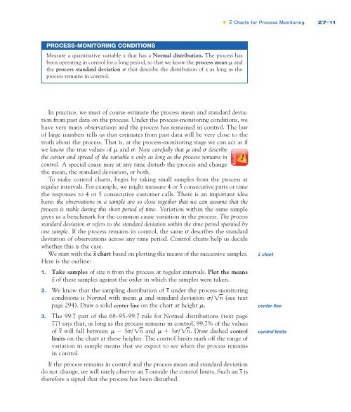
• x Charts for <strong>Process</strong> Monitoring <strong>27</strong>-11<br />
PROCESS-MONITORING CONDITIONS<br />
Measure a quantitative variable x that has a Normal distribution. The process has<br />
been operating in control for a long period, so that we know the process mean and<br />
the process standard deviation that describe the distribution of x as long as the<br />
process remains in control.<br />
In practice, we must of course estimate the process mean and standard deviation<br />
from past data on the process. Under the process-monitoring conditions, we<br />
have very many observations and the process has remained in control. The law<br />
of large numbers tells us that estimates from past data will be very close to the<br />
truth about the process. That is, at the process-monitoring stage we can act as if<br />
we know the true values of and . Note carefully that and describe<br />
the center and spread of the variable x only as long as the process remains in<br />
control. A special cause may at any time disturb the process and change<br />
the mean, the standard deviation, or both.<br />
To make control charts, begin by taking small samples from the process at<br />
regular intervals. For example, we might measure 4 or 5 consecutive parts or time<br />
the responses to 4 or 5 consecutive customer calls. There is an important idea<br />
here: the observations in a sample are so close together that we can assume that the<br />
process is stable during this short period of time. Variation within the same sample<br />
gives us a benchmark for the common cause variation in the process. The process<br />
standard deviation refers to the standard deviation within the time period spanned by<br />
one sample. If the process remains in control, the same describes the standard<br />
deviation of observations across any time period. <strong>Control</strong> charts help us decide<br />
whether this is the case.<br />
We start with the x chart based on plotting the means of the successive samples.<br />
Here is the outline:<br />
1. Take samples of size n from the process at regular intervals. Plot the means<br />
x of these samples against the order in which the samples were taken.<br />
2. We know that the sampling distribution of x under the process-monitoring<br />
conditions is Normal with mean and standard deviation s/ 1n (see text<br />
page 294). Draw a solid center line on the chart at height .<br />
3. The 99.7 part of the 68–95–99.7 rule for Normal distributions (text page<br />
77) says that, as long as the process remains in control, 99.7% of the values<br />
of x will fall between m 3s/ 1n and m 3s/ 1n. Draw dashed control<br />
limits on the chart at these heights. The control limits mark off the range of<br />
variation in sample means that we expect to see when the process remains<br />
in control.<br />
If the process remains in control and the process mean and standard deviation<br />
do not change, we will rarely observe an x outside the control limits. Such an x is<br />
therefore a signal that the process has been disturbed.<br />
x _ chart<br />
center line<br />
control limits


