5.4 Rate of Change of a Rational FunctionâThe Quotient Rule
5.4 Rate of Change of a Rational FunctionâThe Quotient Rule
5.4 Rate of Change of a Rational FunctionâThe Quotient Rule

Create successful ePaper yourself
Turn your PDF publications into a flip-book with our unique Google optimized e-Paper software.
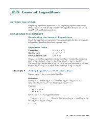
<strong>5.4</strong> <strong>Rate</strong> <strong>of</strong> <strong>Change</strong> <strong>of</strong> a <strong>Rational</strong><br />
Function—The <strong>Quotient</strong> <strong>Rule</strong><br />
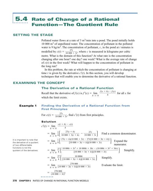
SETTING THE STAGE<br />
Polluted water flows at a rate <strong>of</strong> 3 m 3 /min into a pond. The pond initially holds<br />
10 000 m 3 <strong>of</strong> unpolluted water. The concentration <strong>of</strong> pollutant in the polluted<br />
water is 9 kg/m 3 . The concentration <strong>of</strong> pollutant, c, in the pond at t minutes is<br />
27t<br />
modelled by c(t) 10 00<br />
, where c is measured in kilograms per cubic<br />
0 3t<br />
metre. What is the domain <strong>of</strong> this function? At what rate is the concentration<br />
changing after one hour? one day? one week? What is the average rate <strong>of</strong> change<br />
<strong>of</strong> c(t) in the first week? What will happen to the concentration <strong>of</strong> pollutant in<br />
the long run?<br />
In this problem, the rate at which the concentration <strong>of</strong> pollutant is changing at<br />
time t is given by the derivative c′(t). In this section, you will develop<br />
techniques that will enable you to determine the derivative <strong>of</strong> a rational function.<br />
EXAMINING THE CONCEPT<br />
The Derivative <strong>of</strong> a <strong>Rational</strong> Function<br />
Recall that the derivative <strong>of</strong> f (x) is f ′(x) lim<br />
h → 0<br />
which the limit exists.<br />
f (x h) f (x)<br />
h<br />
for all x for<br />
Example 1<br />
It is important to note that<br />
the derivative <strong>of</strong> a quotient<br />
<strong>of</strong> two differentiable<br />
functions is not the<br />
quotient <strong>of</strong> the derivatives.<br />
Finding the Derivative <strong>of</strong> a <strong>Rational</strong> Function from<br />
First Principles<br />
27t<br />
For c(t) 10 00<br />
, find c′(t) from first principles.<br />
Solution<br />
c′(t) lim<br />
h → 0<br />
lim<br />
h → 0<br />
lim<br />
h → 0<br />
lim 2<br />
h → 0 h<br />
lim 2<br />
h → 0 h<br />
lim<br />
h → 0<br />
<br />
0 3t<br />
c(t h) c(t)<br />
h<br />
1<br />
h <br />
27(t h)<br />
27t<br />
10 000 3(t h) 10 00 0 3t<br />
1<br />
h <br />
27(t h)(10 000 3t) 27t[10 000 3(t h)]<br />
<br />
[10 000 3(t h)](10 000 3t)<br />
Find a common denominator.<br />
Expand the<br />
numerator.<br />
7 Simplify.<br />
7 <br />
10 000h<br />
Simplify.<br />
270 000<br />
<br />
[10 000 3(t h)](10 000 3t)<br />
270 000<br />
<br />
(10 000 3t)<br />
2<br />
10 000t 3t 2 10 000h 3ht (10 000t 3t 2 3ht)<br />
[10 000 3(t h)](10 000 3t)<br />
[10 000 3(t h)](10 000 3t)<br />
Evaluate the limit.<br />
378 CHAPTER 5 RATES OF CHANGE IN RATIONAL FUNCTION MODELS
There is a simpler way <strong>of</strong> finding the derivative for a rational function.<br />
Let h(x) <br />
The <strong>Quotient</strong> <strong>Rule</strong> for Derivatives<br />
f (x)<br />
g(x)<br />
. If both f ′(x) and g′(x) exist, the derivative <strong>of</strong> h(x) is<br />
The rule in words: The<br />
derivative <strong>of</strong> the top times<br />
the bottom minus the<br />
derivative <strong>of</strong> the bottom<br />
times the top all over the<br />
bottom squared.<br />
f ′(x)g(x) g′(x)f (x)<br />
[g(x)]<br />
2<br />
h′(x) , where g(x) ≠ 0.<br />
In Leibniz notation, d<br />
d<br />
x<br />
f (x)<br />
g(x)<br />
d<br />
f<br />
dx<br />
(x) g(x) d<br />
d<br />
g(x) x<br />
f (x)<br />
, g(x) ≠ 0.<br />
[g(x)]<br />
2<br />
Pro<strong>of</strong><br />
The rule for finding the derivative <strong>of</strong> the quotient <strong>of</strong> two functions follows from<br />
the product rule for derivatives. Suppose that there are functions f and g, and<br />
that g(x) 0. Then,<br />
f (x)<br />
g(x)<br />
defines a quotient <strong>of</strong> the two functions.<br />
Let h(x) Multiply both sides by g(x).<br />
g(x)h(x) f (x)<br />
g′(x)h(x) h′(x)g(x) f ′(x)<br />
Differentiate both sides with respect to x.<br />
Solve for h′(x).<br />
h′(x) Substitute h(x) .<br />
<br />
h′(x) <br />
f (x)<br />
g(x)<br />
f ′(x) g′(x)h(x)<br />
g(x)<br />
f ( x)<br />
f ′(x) g′(x) <br />
g ( x)<br />
<br />
g(x)<br />
f ′(x)g(x) g′(x)f (x)<br />
<br />
[g(x)]<br />
2<br />
f (x)<br />
g(x)<br />
Multiply both the numerator and the<br />
denominator by g(x).<br />
Example 2<br />
Technology Help:<br />
For help with<br />
using the numerical<br />
derivative operation,<br />
nDeriv(, see page 595<br />
<strong>of</strong> the Technology<br />
Appendix.<br />
Using the <strong>Quotient</strong> <strong>Rule</strong><br />
Find the derivative <strong>of</strong> each rational function using the quotient rule. Verify with<br />
graphing technology.<br />
(a) y 2 x 5<br />
x<br />
(b) y 3 3<br />
(c) y <br />
3x<br />
1<br />
1 4x<br />
2<br />
x 2<br />
<br />
(x 2)(x 3)<br />
Solution<br />
Use the quotient rule to find the derivative. To verify, graph the derivative<br />
function you found with the TI-83 Plus by entering the function into Y1 <strong>of</strong> the<br />
equation editor. Then enter the numerical derivative <strong>of</strong> the original function as<br />
Y2. Both functions should yield the same graph.<br />
<strong>5.4</strong> RATE OF CHANGE OF A RATIONAL FUNCTION—THE QUOTIENT RULE 379
(a) Apply the quotient rule with f (x) 2x 5 and g(x) 3x 1.<br />
dy<br />
d<br />
<br />
x<br />
<br />
<br />
<br />
(b) f (x) x 3 3 and g(x) 1 4x 2<br />
dy<br />
d<br />
<br />
x<br />
<br />
<br />
<br />
<br />
(c) Here f (x) x 2 and g(x) (x 2)(x 3). Use the product rule to find g′(x).<br />
dy<br />
d<br />
<br />
x<br />
<br />
<br />
<br />
<br />
<br />
f ′(x)g(x) g′(x)f (x)<br />
<br />
[g(x)]<br />
2<br />
2(3x 1) (3)(2x 5)<br />
<br />
(3x 1) 2<br />
6x 2 6x 15<br />
<br />
(3x 1)<br />
2<br />
17<br />
(3x 1)<br />
2<br />
f ′(x)g(x) g′(x)f (x)<br />
<br />
[g(x)]<br />
2<br />
(3x 2 )(1 4x 2 ) (x 3 3)(8x)<br />
<br />
(1 4x 2 ) 2<br />
3x 2 12x 4 8x 4 24x<br />
<br />
(1 4x 2 ) 2<br />
4x 4 3x 2 24x<br />
<br />
(1 4x 2 ) 2<br />
x(4x 3 3x 24)<br />
<br />
(1 4x 2 ) 2<br />
f ′(x)g(x) g′(x)f (x)<br />
<br />
[g(x)]<br />
2<br />
(2x)(x 2)(x 3) [(1)(x 3) (x 2)(1)]x 2<br />
<br />
[(x 2)(x 3)] 2<br />
(2x)(x 2 x 6) x 2 (2x 1)<br />
<br />
(x 2) 2 (x 3) 2<br />
2x 3 2x 2 12x 2x 3 x 2<br />
<br />
(x 2) 2 (x 3) 2<br />
x 2 12x<br />
<br />
(x 2) 2 (x 3) 2<br />
x(x 12)<br />
<br />
(x 2) 2 (x 3) 2<br />
–4.7 ≤ x ≤ 4.7; –5 ≤ y ≤ 5<br />
–4.7 ≤ x ≤ 4.7; –5 ≤ y ≤ 5<br />
–4.7 ≤ x ≤ 4.7; –5 ≤ y ≤ 5<br />
For most functions that are quotients, the derivative function is also a quotient.<br />
Use the quotient rule again to find the second derivative.<br />
Example 3<br />
Finding the Second Derivative <strong>of</strong> a <strong>Rational</strong> Function<br />
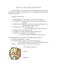
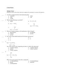
An object moves along a straight line. The object’s position, s, at t seconds is<br />
5t<br />
modelled by s(t) t 2 . When does the object change direction? What is its<br />
1<br />
acceleration at that instant?<br />
380 CHAPTER 5 RATES OF CHANGE IN RATIONAL FUNCTION MODELS
3<br />
2<br />
1<br />
s(t)<br />
s(t) =<br />
5t<br />
t 2 + 1<br />
0 2 4 6 8 10<br />
Solution<br />
When the object changes direction, its velocity, s′(t), changes sign.<br />
The velocity function is v(t) s′(t).<br />
s′(t) <br />
<br />
or<br />
s′(t) 0 when t ±1. But t ≥ 0, so the negative root is inadmissible.<br />
The velocity changes sign when t 1. The object changes direction after<br />
exactly one second.<br />
The acceleration function is a(t) v′(t) s′′(t).<br />
s′′(t) <br />
<br />
<br />
<br />
<br />
<br />
(5)(t 2 1) (2t)(5t)<br />
<br />
( t 2 1 ) 2<br />
5 5t 2<br />
<br />
t 4 2t 2 1<br />
10t(t 4 2t 2 1) (4t 3 4t)(5 5t 2 )<br />
<br />
(t 4 2t 2 1) 2<br />
10t 5 20t 3 10t (20t 3 20t 5 20t 20t 3 )<br />
<br />
[(t 2 1) 2 ] 2<br />
10t 5 20t 3 30t<br />
<br />
(t 2 1) 4<br />
10t(t 4 2t 2 3)<br />
<br />
(t 2 1) 4<br />
10t(t 2 3)(t 2 1)<br />
<br />
(t 2 1) 4<br />
10t(t 2 3)<br />
(t 2 1) 3<br />
1 3)<br />
5(1 t)(1 t)<br />
<br />
t 4 2t 2 1<br />
Simplify.<br />
Factor.<br />
Simplify.<br />
Therefore, s′′(1) 10( ,<br />
( 2)<br />
3<br />
or 2.5.<br />
The object’s acceleration at the instant it changes direction is 2.5 units/s 2 .<br />
t<br />
Graph the position function. When t 1, the object has stopped<br />
briefly. Before t 1, the object was moving away from a point. After<br />
t 1, the object is moving toward the point. Velocity is represented<br />
by the slopes <strong>of</strong> tangent lines to this graph. At the maximum point on<br />
the graph, the slope <strong>of</strong> the tangent line is 0. The velocity is decreasing<br />
before t 1. And the velocity is decreasing after t 1. The graph is<br />
concave down at its peak. The acceleration is negative.<br />
Example 4<br />
Analyzing the Pollution Problem<br />
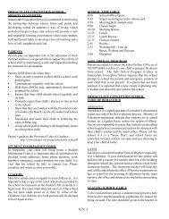
Recall the original problem in Setting the Stage:<br />
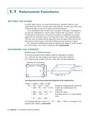
Polluted water flows at a rate <strong>of</strong> 3 m 3 /min into a pond. The pond initially<br />
holds 10 000 m 3 <strong>of</strong> unpolluted water. The initial concentration <strong>of</strong> pollutant in<br />
the polluted water is 9 kg/m 3 . The concentration <strong>of</strong> pollutant, c, in the pond at<br />
27t<br />
t minutes is modelled by c(t) 10 00<br />
.<br />
0 3t<br />
(a) What is the domain <strong>of</strong> this function?<br />
(b) At what rate is the concentration changing after one hour? one day?<br />
one week?<br />
<strong>5.4</strong> RATE OF CHANGE OF A RATIONAL FUNCTION—THE QUOTIENT RULE 381
10<br />
8<br />
6<br />
4<br />
You could find these values<br />
more quickly using nDeriv(,<br />
which is accurate to five<br />
decimal places.<br />
c(t)<br />
c(t) =<br />
27t<br />
10 000 + 3t<br />
2<br />
t<br />
0 2000 4000 6000 8000 10 000<br />
(c) What is the average rate <strong>of</strong> change <strong>of</strong> c(t) in the first week?<br />
(d) What will happen to the concentration <strong>of</strong> pollutant in the long run?<br />
Solution<br />
27t<br />
(a) Since t represents time, the domain <strong>of</strong> c(t) 10 00<br />
is restricted to all<br />
0 3t<br />
real numbers greater than or equal to 0, {t ⎢ t ≥ 0, t ∈ R}.<br />
(b) Find the derivative.<br />
c′(t) <br />
Simplify.<br />
<br />
27(10 000 3t) (3)(27t)<br />
<br />
(10 000 3t) 2<br />
270 000<br />
<br />
(10 000 3t)<br />
2<br />
At 1 h, t 60, and c′(60) 0.0026.<br />
At 1 h, the concentration is increasing at about 0.0026 kg/m 3 /min.<br />
After one day, t 1440, and c′(1440) 0.0013.<br />
After one day, the concentration is increasing at about 0.0013 kg/m 3 /min.<br />
After one week, t 10 080, and c′(10 080) 0.0002.<br />
After one week, the concentration is increasing at about 0.0002 kg/m 3 /min.<br />
The rate at which the concentration is increasing decreases over time.<br />
c(10 080) c(0)<br />
(c) The average rate <strong>of</strong> change <strong>of</strong> c(t) in the first week is <br />
10 080 0<br />
, or<br />
about 0.0007 kg/m 3 /min.<br />
(d) To determine what happens to the concentration <strong>of</strong> pollutant in the long run,<br />
find lim c(t).<br />
t → ∞<br />
lim<br />
t → ∞<br />
27t<br />
10 00 0 3t<br />
lim<br />
t → ∞<br />
27<br />
<br />
0 3<br />
27 t<br />
<br />
t<br />
<br />
10 000<br />
3 t<br />
<br />
t t<br />
9<br />
The concentration will approach the concentration <strong>of</strong> the polluted water<br />
entering the pond.<br />
Of course, this conclusion assumes that the pond has an infinite<br />
capacity, which is not a reasonable assumption!<br />
The pond would actually overflow into the surrounding area and the<br />
water would drain away into the ground or into any nearby creeks,<br />
carrying the pollution farther afield.<br />
Graph concentration versus time. The slopes <strong>of</strong> the tangent lines<br />
decrease over time. The curve seems to approach a limiting value.<br />
382 CHAPTER 5 RATES OF CHANGE IN RATIONAL FUNCTION MODELS
CHECK, CONSOLIDATE, COMMUNICATE<br />
1. Use an example to show that the derivative <strong>of</strong> a rational function is not<br />
the same as the quotient <strong>of</strong> the derivatives <strong>of</strong> its numerator and<br />
denominator.<br />
2. Compare the quotient rule to the product rule. What is similar about the<br />
two rules? What is different?<br />
3. Why might you need to find the first and second derivatives <strong>of</strong> a rational<br />
function? Give an example <strong>of</strong> a rational function. Then find the first and<br />
second derivatives.<br />
KEY IDEAS<br />
• The derivative <strong>of</strong> a quotient <strong>of</strong> two differentiable functions is not the<br />
quotient <strong>of</strong> their derivatives.<br />
• The quotient rule is a rule for finding the derivative <strong>of</strong> a rational<br />
function.<br />
f (x)<br />
Let h(x) g(x)<br />
. If both f ′(x) and g′(x) exist, the derivative <strong>of</strong> h(x) is<br />
h′(x) where g(x) ≠ 0.<br />
• The quotient rule in Leibniz notation is<br />
, g(x) ≠ 0.<br />
d<br />
d<br />
x<br />
f ′(x)g(x) g′(x)f (x)<br />
[g(x)]<br />
2<br />
d<br />
f<br />
dx<br />
(x) g(x) d<br />
f (x)<br />
d<br />
g(x) x<br />
f (x)<br />
g(x) [g(x)]<br />
2<br />
<strong>5.4</strong> Exercises<br />
A<br />
1. Find the derivative <strong>of</strong> each rational function from first principles.<br />
x<br />
(a) f (x) 3 <br />
(b) g(x) x <br />
<br />
2 (c) h(x) <br />
x<br />
1 x<br />
2. Use the quotient rule to find f ′(x) for each function.<br />
(a) f (x) x <br />
<br />
3<br />
x 3<br />
(b) f (x) <br />
(c) f (x) <br />
(d) f (x) <br />
(e) f (x) <br />
x 3 2x<br />
x 2 x 1<br />
(f) f (x) <br />
3x 4<br />
x 2 6<br />
(x 4)(x 5)<br />
<br />
2x(x 3)<br />
x<br />
3<br />
1 x<br />
ax b<br />
cx d<br />
3x 2 2<br />
x<br />
(g) f (x) <br />
(i) f (x) <br />
x 2 1<br />
2x 3<br />
1 x 4<br />
x<br />
2<br />
(h) f (x) <br />
5x 4 9<br />
x 2<br />
(j) f (x) 5 1 x <br />
x 3<br />
<strong>5.4</strong> RATE OF CHANGE OF A RATIONAL FUNCTION—THE QUOTIENT RULE 383
3. Verify your answers for question 2 by graphing Y1 f ′(x) and<br />
Y2 nDeriv f (x) in the same window.<br />
dy<br />
4. Find d<br />
.<br />
x<br />
(a) y <br />
(b) y <br />
(c) y <br />
(d) y <br />
5. When asked to find the derivative <strong>of</strong> f (x) x<br />
2 , Vassili used the<br />
quotient rule. Instead <strong>of</strong> using the quotient rule, Kelly divided each term in<br />
the numerator by the denominator and then simplified. Then she found the<br />
derivative <strong>of</strong> each term. Find the derivative using each method. Explain<br />
which method you prefer, and why.<br />
6. Knowledge and Understanding: Find the equation <strong>of</strong> the tangent to the<br />
x<br />
graph <strong>of</strong> f (x) 3 <br />
at the point where x 1.<br />
2x<br />
7. Find an equation for the tangent to the graph <strong>of</strong> the function at the given<br />
value <strong>of</strong> x.<br />
x<br />
(a) f (x) x <br />
; x 5<br />
(b) f (x) 2 5<br />
3<br />
x 5<br />
x 1<br />
; x 1<br />
8. Find the point(s) where the tangent to the curve is horizontal.<br />
(a) f (x) <br />
(b) f (x) <br />
x 6<br />
(x 1)<br />
2<br />
5x 3<br />
2(x 3)<br />
(x 1)(x 4)<br />
(x 2)<br />
x 5<br />
<br />
(3x 1)(3x 2)<br />
5x<br />
x 2 1<br />
x 2 2x 4<br />
x 2 4<br />
9. An object moves along a straight line. The object’s position at time t is<br />
given by s(t). Find the position, velocity, acceleration, and speed at the<br />
specified time.<br />
2t<br />
(a) s(t) t <br />
; t 3<br />
3<br />
5<br />
(b) s(t) t t <br />
; t 1<br />
2<br />
10. Communication: An object moves along a straight line so that its position,<br />
t<br />
s, at t seconds is given by s(t) 2 2t 5<br />
t 2<br />
. Does the object change<br />
direction at any time? Justify your answer.<br />
11. The position, s, <strong>of</strong> an object that moves in a straight line at time t is given<br />
by s(t) . Determine when the object changes direction.<br />
t<br />
t 2 8<br />
x 5 2x<br />
384 CHAPTER 5 RATES OF CHANGE IN RATIONAL FUNCTION MODELS
12. Salt water has a concentration <strong>of</strong> 10 g <strong>of</strong> salt per litre. The salt water flows<br />
into a large tank that initially holds 500 L <strong>of</strong> pure water. Twenty litres <strong>of</strong> the<br />
salt water flow into the tank per minute. Show that the concentration <strong>of</strong> salt,<br />
10t<br />
c, in the tank at t minutes is given by c(t) 25<br />
, where c is measured in<br />
t<br />
grams per litre. What is the rate <strong>of</strong> change <strong>of</strong> c with respect to t?<br />
13. Application: The concentration, c, <strong>of</strong> a drug in the blood t hours after the<br />
5t<br />
drug is taken orally is given by c(t) 2t 2 . When does the concentration<br />
7<br />
reach its maximum value?<br />
14. At a manufacturing plant, productivity is measured by the number <strong>of</strong> items,<br />
p, produced per employee per day over the previous 10 years.<br />
25t<br />
Productivity is modelled by p(t) t<br />
, where t is the number <strong>of</strong> years<br />
1<br />
measured from 10 years ago. Determine the rate <strong>of</strong> change <strong>of</strong> p with respect<br />
to t.<br />
dy<br />
15. Find d<br />
for y <br />
x<br />
positive.<br />
x 2 1<br />
2x 2 1<br />
dy<br />
. Determine the values <strong>of</strong> x for which d<br />
is<br />
x<br />
C<br />
16. Functions u and v are differentiable functions <strong>of</strong> x, and y u . Determine<br />
v<br />
dy<br />
d x<br />
from first principles.<br />
17. The radius <strong>of</strong> a circular juice blot on a piece <strong>of</strong> paper towel t seconds after<br />
it was first seen is modelled by r(t) 1 2t<br />
, where r is measured in<br />
1 t<br />
centimetres. Calculate<br />
(a) the radius <strong>of</strong> the blot when it was first observed<br />
(b) the time at which the radius <strong>of</strong> the blot was 1.5 cm<br />
(c) the rate <strong>of</strong> increase <strong>of</strong> the area <strong>of</strong> the blot when the radius was 1.5 cm<br />
(d) According to this model, will the radius <strong>of</strong> the blot ever reach 2 cm?<br />
Explain your answer.<br />
(7t<br />
9)<br />
18. Check Your Understanding: The function P(t) 30 models the<br />
3t<br />
2<br />
population, in thousands, <strong>of</strong> a town t years since 1985. Determine the first<br />
and second derivatives. What information do these two derivative functions<br />
give? Explain using numerical examples. Describe the population <strong>of</strong> this<br />
town.<br />
19. Find the equations <strong>of</strong> the tangents from the origin to the graph <strong>of</strong> y x .<br />
x<br />
Sketch the function and the tangent lines.<br />
8<br />
6<br />
20. Thinking, Inquiry, Problem Solving: Choose a simple polynomial function<br />
in the form f (x) ax b. Use the quotient rule to find the derivative <strong>of</strong><br />
1<br />
the reciprocal function ax<br />
. Repeat for other polynomial functions, and<br />
b<br />
1<br />
devise a rule for finding the derivative <strong>of</strong> f (x)<br />
. Confirm your rule using first<br />
principles.<br />
<strong>5.4</strong> RATE OF CHANGE OF A RATIONAL FUNCTION—THE QUOTIENT RULE 385
ADDITIONAL ACHIEVEMENT CHART QUESTIONS<br />
Knowledge and Understanding: Determine the derivative for f (x) x 2 .<br />
1<br />
Verify your answer by graphing the derivative and using nDeriv( for f (x).<br />
Application: The position function <strong>of</strong> a particle moving in a straight line is<br />
s(t) , where 0 ≤ t ≤ 10. When is the velocity a maximum?<br />
10t 2<br />
32 t<br />
2<br />
x 2 1<br />
Pierre de Fermat<br />
(1601–1665)<br />
Pierre de Fermat<br />
treated mathematics as<br />
an interesting hobby,<br />
rather than as a<br />
pr<strong>of</strong>ession. He made<br />
contributions in<br />
calculus, number<br />
theory, and optics. Do<br />
some research on<br />
Fermat’s Last Theorem.<br />
Why is it appropriate<br />
that this note on<br />
Fermat is in the<br />
margin <strong>of</strong> a math text?<br />
Thinking, Inquiry, Problem Solving: The graph <strong>of</strong> f (x) <br />
ax b<br />
<br />
(x 1)(x 4)<br />
horizontal tangent line at (2, 1). Find a and b. Check using a graphing<br />
calculator.<br />
has a<br />
Communication: A shirt manufacturer has records that show that the unit cost,<br />
C, per shirt produced by a worker is given by C(t) 15 0.6t<br />
, where t is the<br />
5t<br />
number <strong>of</strong> hours worked per day. Find approximate values for C′′(t) at t 1, 3,<br />
5, and 7. Describe what the numbers tell you about the cost per shirt.<br />
The Chapter Problem<br />
Designing a Settling Pond<br />
Apply what you learned in this section to answer these questions about<br />
The Chapter Problem on page 342.<br />
CP10. Determine the first and second derivatives <strong>of</strong> the first<br />
concentration function.<br />
CP11. At what rate is the concentration changing after one hour? one<br />
day? one week? What is the average rate <strong>of</strong> change in the first<br />
week?<br />
CP12. Repeat questions CP10 and CP11 for the second concentration<br />
function.<br />
386 CHAPTER 5 RATES OF CHANGE IN RATIONAL FUNCTION MODELS