download

More documents

Recommendations

Info

( ∂ u ∂ ) 2 , ( ∂ u ∂ ) 2 , ( ∂ u ∂ ) 2 , ( ∂u ∂ ) 2 1 x 1 3 x 1 1 x 3 3 x 3 along the duct centreline is plotted in Figure 6. The gradients have been evaluated by fitting a line between the values of f ii (∆x j ) for ∆x j varying between 0.1-0.6 mm. This corresponds to a range of 1-5 Kolgomorov scale η. The best fitting line has been found maximising the correlation factor R of the linear interpolation. Regardless of the experimental scatter of the gradient values, the isotropic conditions illustrated in equations (3), (4) are satisfactorily achieved. (∂u/∂x) 2 [ s -2 ] 2200 2000 1800 1600 1400 1200 1000 800 600 400 0.5 U 1 (∂q 2 /∂x 1 )(1/15 ν) (∂u 1 /∂x 1 ) 2 (∂u 1 /∂x 3 ) 2 (∂u 3 /∂x 3 ) 2 (∂u 3 /∂x 1 ) 2 (1/U 2 1 )(∂u 1 /∂t) 2 200 18 20 22 24 26 28 30 32 34 36 38 x 1 /M Figure 6 Comparison between the values assumed by the spatial gradients directly measured (red, black, blue and green circles) and the ( ∂u ∂ ) 2 hypothesis (triangles). 1 x 1 gradient calculated from the kinetic energy decay (violet line) and from Taylor's In Figure 6 the values of the spatial gradients measured directly are compared with the values of ( ∂u ∂ ) 2 1 x 1 calculated with the kinetic energy decay and with Taylor hypothesis. The latter gradients have been calculated applying the slotting technique (Van Maanen & Tummers (1996)), normally used to determine the autocorrelation coefficient. In the present work the technique is used to evaluate the f ii coefficients for different time intervals ∆t. Even in this case the time coincidence window used is 0.03 ms. The different methods implemented show a good agreement. A comparison between the values of the scaled dissipation ( ε M/ U 1 ) from the present and previous works is shown in Figure 7. The dissipation values are calculated from the kinetic energy decay. The coefficients A and n of the kinetic energy decay have been taken from Mohamed & LaRue (1990) who, as already mentioned, revisited some of the earliest work on grid turbulence flow. The non dimensional dissipation values have been plotted for X 1 /M in the range of 20-40 M. The values of ε M/ U 1 shown in Figure 7 differ by a large amount (46 % difference between the values of the curves located furthest away from each other). Considering the high values of Re M used in some of the past works, it is possible that for some of them the isotropic region commenced somewhere in the range or even at higher distances from the grid, but this do not affect the validity of the graph. In fact the dissipation decaying coefficients (1+n) of the curves plotted vary by small amounts (2.26-2.35), so that can be assumed that all the curves remain parallel to each other and their differences do not become smaller for higher values of x 1 /M. The high difference between the scaled values 3 ε M/ U 1 is due to the substantial variation of A (0.0364-0.0664) from one work to the other. From Figure 7 it can 3 be observed that the values of ε M/ U 1 of the present work lie between the curves of the previous works. 3 3 8
ε M/ U 1 3 1E-4 Larue Re M = 6000 " Re M = 10000 " Re M = 14000 " Re M = 12000 Wyatt(1955) Re M = 11000 Van Atta & Chen (1969) Re M = 25600 Comte-Bellot & Corsin (1966) Re M = 34000 Sreenivasan et al. (1980) Re M = 7400 Uberoi (1963) Re M = 10000 Uberoi & Wallis (1967) Re M =29000 Sirivat & Warhaft (1983) Re M =8750 present data Re M =5150 1E-5 20 25 30 35 40 45 50 55 60 x 1 /M Figure 7 Comparison between the values assumed by the dimensionless dissipation previous works. ε M/ U 1 3 in the present and in The comparison between the values of the dissipation calculated from the decay of kinetic energy and from the direct estimation of the gradients have been illustrated in Figure 1. According to the isotropic relation (4), the contribution to dissipation due to the spatial gradient ( u ∂ ) 2 gradients ( ∂ u ∂ ) 2 and ( u ∂ ) 2 1 x 3 ∂ . 3 x 1 5. 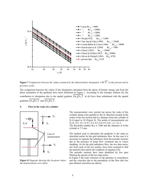Flow in the wake of a cylinder ∂ in (6) have been substituted with the spatial 3 x 2 X 1 /d X 1 X 3 The measurements were carried out across the wake of the cylinder along a line parallel to the X 3 direction located in the centre of the test section and at a distance from the cylinder of X 1 /d equal to 10 (Figure 8). The points of measurements are X 3 /d: -0.2, -0.1, 0, 0.1, 0.2, 0.3, 0.4, 0.5, 0.8, 1.2, 1.6, 2. The Reynolds number Re d is 7200 and the diameter d of the cylinder is 7.2 mm. Line of measurement X 2 X 3 Figure 8 Diagram showing the locations where the measurements were taken The method used to determine the gradients is the same as described earlier for the grid turbulence flow. In this case it is necessary to separate the turbulence from the periodic motions due to the presence of mean flow variations due to vortex shedding. As for the grid turbulence flow, the two data series, one from each of the two probes, have been scanned to find the particles that satisfy the condition of equation (10). The periodic motions have been identified by low pass filtering the spectra of the two data series. In Figure 9 the total velocities of the particles in coincidence and the velocities due to the periodicity of the flow (the low pass filtered velocities) are shown. 9
Page 1 and 2: Direct Measurement of the Turbulent
Page 3 and 4: Mohamed & LaRue (1990) performed an
Page 5 and 6: Table 3. Focal length and control v
Page 7: the two probes are aligned at the s
Page 11 and 12: 6. Conclusions A LDA method to meas

download

You also want an ePaper? Increase the reach of your titles

Delete template?

Save as template?