Homework 3 (pdf) - Geotechnical Earthquake Engineering
Homework 3 (pdf) - Geotechnical Earthquake Engineering
Homework 3 (pdf) - Geotechnical Earthquake Engineering

Create successful ePaper yourself
Turn your PDF publications into a flip-book with our unique Google optimized e-Paper software.
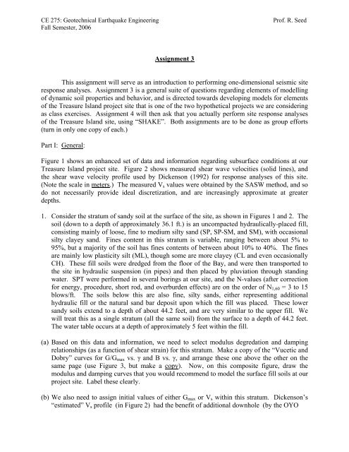
CE 275: <strong>Geotechnical</strong> <strong>Earthquake</strong> <strong>Engineering</strong><br />
Fall Semester, 2006<br />
Prof. R. Seed<br />
Assignment 3<br />
This assignment will serve as an introduction to performing one-dimensional seismic site<br />
response analyses. Assignment 3 is a general suite of questions regarding elements of modelling<br />
of dynamic soil properties and behavior, and is directed towards developing models for elements<br />
of the Treasure Island project site that is one of the two hypothetical projects we are considering<br />
as class exercises. Assignment 4 will then ask that you actually perform site response analyses<br />
of the Treasure Island site, using “SHAKE”. Both assignments are to be done as group efforts<br />
(turn in only one copy of each.)<br />
Part I: General:<br />
Figure 1 shows an enhanced set of data and information regarding subsurface conditions at our<br />
Treasure Island project site. Figure 2 shows measured shear wave velocities (solid lines), and<br />
the shear wave velocity profile used by Dickenson (1992) for response analyses of this site.<br />
(Note the scale in meters.) The measured V s values were obtained by the SASW method, and so<br />
do not necessarily provide ideal discretization, and are increasingly approximate at greater<br />
depths.<br />
1. Consider the stratum of sandy soil at the surface of the site, as shown in Figures 1 and 2. The<br />
soil (down to a depth of approximately 36.1 ft.) is an uncompacted hydraulically-placed fill,<br />
consisting mainly of loose, fine to medium silty sand (SP, SP-SM, and SM), with occasional<br />
silty clayey sand. Fines content in this stratum is variable, ranging between about 5% to<br />
95%, but a majority of the soil has fines contents of between about 10% to 40%. The fines<br />
are mainly low plasticity silt (ML), though some are more clayey (CL and even occasionally<br />
CH). These fill soils were dredged from the floor of the Bay, and were then transported to<br />
the site in hydraulic suspension (in pipes) and then placed by pluviation through standing<br />
water. SPT were performed in several borings at our site, and the N-values (after correction<br />
for energy, procedure, short rod, and overburden effects) are on the order of N 1,60 = 3 to 15<br />
blows/ft. The soils below this are also fine, silty sands, either representing additional<br />
hydraulic fill or the natural sand bar deposit upon which the fill was placed. These lower<br />
sandy soils extend to a depth of about 44.2 feet, and are very similar to the upper fill. We<br />
will treat this as a single stratum (all the same soil) from the surface to a depth of 44.2 feet.<br />
The water table occurs at a depth of approximately 5 feet within the fill.<br />
(a) Based on this data and information, we need to select modulus degredation and damping<br />
relationships (as a function of shear strain) for this stratum. Make a copy of the “Vucetic and<br />
Dobry” curves for G/G max vs. γ and B vs. γ, and arrange these one above the other on the<br />
same page (use Figure 3, but make a copy). Now, on this composite figure, draw the<br />
modulus and damping curves that you would recommend to model the surface fill soils at our<br />
project site. Label these clearly.<br />
(b) We also need to assign initial values of either G max or V s within this stratum. Dickenson’s<br />
“estimated” V s profile (in Figure 2) had the benefit of additional downhole (by the OYO
suspension logger method) V s data that will not be available to us. (Dickenson used the two<br />
V s data sets, as well as a suite of empirical correlations, and then selected his V s profile.)<br />
(i)<br />
(ii)<br />
Assume reasonable unit weights for the upper fill, and calculate and plot a profile of<br />
σ v΄ vs. depth within the upper 42 feet.<br />
At depths of 10, 20, and 40 feet, estimate G max and V s using the correlations of<br />
• Seed et al., 1984<br />
• Imai and Tonouchi, 1982<br />
• Sykora and Stokoe, 1983<br />
• Hardin, 1983 (Estimate that OCR ≈ 1 to 1.5 for these upper sands)<br />
(iii)<br />
(iv)<br />
(v)<br />
Plot these profiles of V s vs. depth, and on the same figure also plot the measured V s<br />
data (in the upper sands) from Figure 2.<br />
Now we have to decide how to sub-divide our soil into sub-layers. Based on the V s<br />
estimates thus far, and your notion of frequency needs and resulting wavelengths,<br />
sub-divide the upper sands into X sublayers (and explain your selection of X.)<br />
Now, based on all of this, select proposed V s values for use within each of these sublayers<br />
in your SHAKE analyses. On a full-depth profile, plot V s vs. depth. (You will<br />
continue this figure right down to the rock by the time you have finished this<br />
assignment, so scale this figure accordingly.)<br />
2. Now consider the deposit of clayey soils immediately underlying the upper sands (from a<br />
depth of about 44.2 feet to about 95.4 feet.) This soil is San Francisco Bay Mud, a Holocene<br />
deposit of marine clay and silty clay (CH), with occasional silty and sandy lenses. The Bay<br />
Mud is a nearly normally consolidated clay (beneath the fill at our site), and is of low<br />
strength. It is also “sensitive”, and highly compressible under long-term loads too. The Bay<br />
Mud at our site has a Plasticity Index of PI ≈ 45 to 55%.<br />
(a) We will begin by estimating the undrained shear strength of the Bay Mud. Based on<br />
laboratory testing of “undisturbed” samples (UU Triaxial tests), and in-situ vane shear tests<br />
(corrected with Bjerrum’s correction), and one-dimensional laboratory consolidation tests, it<br />
appears that this deposit is essentially normally consolidated (OCR = 1.0 to 1.3), and that<br />
S u /P = 0.32 to 0.35. Does this seem reasonable?<br />
(b) Assuming a reasonable value for the unit weight of the Bay Mud, continue your profile of σ v΄<br />
vs. depth down to the base of the Bay Mud (at a depth of 95.4 feet.) The Bay Mud is lighter<br />
than the sandy fills, and a good average estimate of unit weight is γ sat = 94 to 100 lb/ft 3 . How<br />
would the unit weight vary with depth? Would this matter for our purposes?
(c) Now, based on this effective stress profile, and S u /P = 0.32 to 0.35, plot your estimate of S u<br />
vs. depth within the Bay Mud.<br />
(d) Now, using Dickenson’s recommended correlation between S u and V s , plot your estimated<br />
profile of V s vs. depth within the Bay Mud. On the same plot, also plot the measured V s data<br />
(from Figure 2.)<br />
(e) Based on this, and considering wavelengths and frequencies, decide how to sub-divide the<br />
Bay Mud stratum into sub-layers. Explain your rationale.<br />
(f) Finally, based on all of this, select recommended values of V s within each sublayer, and plot<br />
this vs. depth (on the same figure with your chosen profile of V s within the upper sands.)<br />
(g) We will, of course, also need modulus degredation and damping curves. Make another copy<br />
of the Vucetic and Dobry curves (Figure 3.) Onto this, plot the material-specific curves for<br />
Bay Mud recommended by Dickenson (Figure 4.) How do these compare with the Vucetic<br />
and Dobry data set (at similar PI)?<br />
3. Now, repeat the above exercises for the deeper soils (down to a depth of 298.9 feet.) The<br />
following data and information will be helpful.<br />
(a) The Bay Mud is underlain by a deposit of medium to dense, fine to medium sand and silty<br />
sand (SP, and SP/SM) to a depth of approximately 135.7 feet. These sands have been in<br />
place for at least the second half of the Holocene period, and have been shaken by many<br />
earthquakes. Based on SPT borings, corrected N-values in these sands are typically on the<br />
order of N 1,60 = 25 to 50 blows/ft. Fines contents vary, but are typically on the order of 5 to<br />
25%, but with occasional thin silt and clay lenses.<br />
(b) These sandy strata are underlain by Old Bay Clays (CH/CL). These are pre-Holocene units,<br />
and are overconsolidated due to Bay level fluctuations and also ageing (and attendant<br />
secondary compression.) It is a bit difficult to get good undrained shear strength data on<br />
these deeper clays, as the samples tend to be disturbed by unloading. The limited data<br />
available to us (from our project borings and testing) suggests that S u is approximately 2,700<br />
to 5,200 lb/ft 2 in this unit, but we are not very confident in this data. We also have the<br />
measured V s data from Figure 2. Think about how V s should vary with depth in this unit.<br />
Also, check the implied ratio of S u /P, and think about OCR and SHANSEP. (OCR appears<br />
to be on the order of about 3 to 7 in this unit.)<br />
(c) The Old Bay Clays are underlain, at a depth of about 248 feet, by very dense sands and<br />
gravelly sands (SP, SW). We don’t have much SPT data here, as the depth is great, the soils<br />
are dense, and the gravels impede the SPT penetrometer. You will have to make your own<br />
guesses. (We do know that this unit is dense to very dense, and expect that N 1,60 values will<br />
be on the order of about 40 to 80 or more.) Remember that we also have measured V s data<br />
(Figure 2), but we are getting rather deep for SASW.
(d) The deep, dense gravelly sands are underlain by additional Old Bay Clays (CH/CL). These<br />
are even older, and so are even stiffer and stronger. Treat these as an extension of the Old<br />
Bay Clay unit from above the gravelly sands. Again, remember that we also have V s data,<br />
but that SASW does not work well in the “shadow” just below a stiffer layer (e.g. the<br />
gravelly sands), and that we are very deep for SASW!<br />
(e) Our site investigations (both borings and testing, as well as SASW) provided essentially no<br />
useful, quantitive data regarding the weathered shale and the harder, more intact sandstone<br />
“bedrock” underlying the deep clays. Refer to Figures 1 and 2. Dickenson assigned Vs =<br />
730 m/sec to the weathered shale, and treated the sandstone as an elastic halfspace with Vs =<br />
1,220 m/sec. Do these values seem reasonable? Now, feel free to choose your own.<br />
4. Finally, prepare a full proposed site profile, divided into sub-layers, for your response<br />
analyses. Show the proposed profile of V s vs. depth, and provide figures showing your<br />
proposed relationships for G/Gmax vs. γ and B vs. γ for each soil and/or “rock” unit,<br />
including the base “rock”.