Linear Systems - ResearchGate
Linear Systems - ResearchGate
Linear Systems - ResearchGate

You also want an ePaper? Increase the reach of your titles
YUMPU automatically turns print PDFs into web optimized ePapers that Google loves.
<strong>Linear</strong> <strong>Systems</strong><br />
John A. Scales<br />
Samizdat<br />
Press
<strong>Linear</strong> <strong>Systems</strong><br />
1<br />
John A. Scales<br />
Colorado School of Mines<br />
jscales@mines.edu<br />
Samizdat Press<br />
Golden · White River Junction
2<br />
Published by the Samizdat Press<br />
Center for Wave Phenomena<br />
Department of Geophysics<br />
Colorado School of Mines<br />
Golden, Colorado 80401<br />
and<br />
New England Research<br />
76 Olcott Drive<br />
White River Junction, Vermont 05001<br />
c○Samizdat Press, 2001<br />
Release 4, April 1, 2001<br />
Samizdat Press publications are available via FTP<br />
from http://samizdat.mines.edu<br />
Permission is given to freely copy these documents.
Contents<br />
1 Simple Harmonic Motion: From Springs to Waves 1<br />
1.1 A Spring and a Mass . . . . . . . . . . . . . . . . . . . . . . . . . . . . . 4<br />
1.1.1 Simple harmonic oscillation . . . . . . . . . . . . . . . . . . . . . 4<br />
1.1.2 Forced motion . . . . . . . . . . . . . . . . . . . . . . . . . . . . . 9<br />
1.1.3 Complex numbers and constant coefficient differential equations . 10<br />
1.1.4 Forced motion with damping . . . . . . . . . . . . . . . . . . . . . 12<br />
1.1.5 Damped transient motion . . . . . . . . . . . . . . . . . . . . . . 16<br />
1.1.6 Another velocity-dependent force: the Zeeman effect . . . . . . . 16<br />
1.2 Two Coupled Masses . . . . . . . . . . . . . . . . . . . . . . . . . . . . . 19<br />
1.2.1 A Matrix Appears . . . . . . . . . . . . . . . . . . . . . . . . . . 21<br />
1.2.2 Matrices for two degrees of freedom . . . . . . . . . . . . . . . . . 23<br />
1.2.3 The energy method . . . . . . . . . . . . . . . . . . . . . . . . . . 24<br />
1.2.4 Matrix form of the coupled spring/mass system . . . . . . . . . . 25<br />
1.3 More on coupled spring/mass lattices . . . . . . . . . . . . . . . . . . . . 31<br />
2 Waves and Modes in One and Two Spatial Dimensions 37<br />
2.1 1-D Separation of Variables: Summary of the Argument . . . . . . . . . . 38<br />
2.2 2-D separation of variables . . . . . . . . . . . . . . . . . . . . . . . . . . 40<br />
2.3 An Example . . . . . . . . . . . . . . . . . . . . . . . . . . . . . . . . . . 43<br />
i
ii<br />
CONTENTS<br />
2.4 Degeneracy . . . . . . . . . . . . . . . . . . . . . . . . . . . . . . . . . . 44<br />
2.5 Pictures of Modes . . . . . . . . . . . . . . . . . . . . . . . . . . . . . . . 46<br />
2.6 Spherical and Cylindrical Harmonics . . . . . . . . . . . . . . . . . . . . 47<br />
2.6.1 separation of variables . . . . . . . . . . . . . . . . . . . . . . . . 50<br />
2.6.2 Properties of Spherical Harmonics and Legendre Polynomials . . . 54<br />
2.7 Exercises . . . . . . . . . . . . . . . . . . . . . . . . . . . . . . . . . . . . 56<br />
2.8 More on vectors . . . . . . . . . . . . . . . . . . . . . . . . . . . . . . . . 65<br />
3 A Little More <strong>Linear</strong> Algebra 71<br />
3.1 <strong>Linear</strong> Vector Spaces . . . . . . . . . . . . . . . . . . . . . . . . . . . . . 71<br />
3.2 Matrices . . . . . . . . . . . . . . . . . . . . . . . . . . . . . . . . . . . . 73<br />
3.3 Some Special Matrices . . . . . . . . . . . . . . . . . . . . . . . . . . . . 76<br />
3.4 Matrix and Vector Norms . . . . . . . . . . . . . . . . . . . . . . . . . . 77<br />
3.5 Projecting Vectors Onto Other Vectors . . . . . . . . . . . . . . . . . . . 78<br />
3.6 <strong>Linear</strong> Dependence and Independence . . . . . . . . . . . . . . . . . . . . 80<br />
3.7 The Four Fundamental Spaces . . . . . . . . . . . . . . . . . . . . . . . . 81<br />
3.7.1 Spaces associated with a linear system Ax = y . . . . . . . . . . . 81<br />
3.7.2 A Geometrical Picture . . . . . . . . . . . . . . . . . . . . . . . . 83<br />
3.8 Matrix Inverses . . . . . . . . . . . . . . . . . . . . . . . . . . . . . . . . 83<br />
3.9 Elementary operations and Gaussian Elimination . . . . . . . . . . . . . 85<br />
3.9.1 Examples . . . . . . . . . . . . . . . . . . . . . . . . . . . . . . . 85<br />
3.10 Least Squares . . . . . . . . . . . . . . . . . . . . . . . . . . . . . . . . . 88<br />
3.10.1 Examples of Least Squares . . . . . . . . . . . . . . . . . . . . . . 91<br />
3.11 Eigenvalues and Eigenvectors . . . . . . . . . . . . . . . . . . . . . . . . 92<br />
3.12 Orthogonal decomposition of rectangular matrices . . . . . . . . . . . . . 96<br />
3.13 Eigenvectors and Orthogonal Projections . . . . . . . . . . . . . . . . . . 98
CONTENTS<br />
iii<br />
3.14 A few examples . . . . . . . . . . . . . . . . . . . . . . . . . . . . . . . . 99<br />
4 Fourier Analysis 105<br />
4.1 Motivation . . . . . . . . . . . . . . . . . . . . . . . . . . . . . . . . . . . 105<br />
4.2 The Fourier Series . . . . . . . . . . . . . . . . . . . . . . . . . . . . . . . 106<br />
4.2.1 Examples . . . . . . . . . . . . . . . . . . . . . . . . . . . . . . . 109<br />
4.3 Superposition and orthogonal projection . . . . . . . . . . . . . . . . . . 111<br />
4.4 The Fourier Integral . . . . . . . . . . . . . . . . . . . . . . . . . . . . . 113<br />
4.4.1 Examples . . . . . . . . . . . . . . . . . . . . . . . . . . . . . . . 115<br />
4.4.2 Some Basic Theorems for the Fourier Transform . . . . . . . . . . 117<br />
4.5 The Sampling Theorem . . . . . . . . . . . . . . . . . . . . . . . . . . . . 119<br />
4.5.1 Aliasing . . . . . . . . . . . . . . . . . . . . . . . . . . . . . . . . 121<br />
4.6 The Discrete Fourier Transform . . . . . . . . . . . . . . . . . . . . . . . 122<br />
4.7 The <strong>Linear</strong> Algebra of the DFT . . . . . . . . . . . . . . . . . . . . . . . 123<br />
4.8 The DFT from the Fourier Integral . . . . . . . . . . . . . . . . . . . . . 124<br />
4.8.1 Discrete Fourier Transform Examples . . . . . . . . . . . . . . . . 126<br />
4.9 Convergence Theorems . . . . . . . . . . . . . . . . . . . . . . . . . . . . 127<br />
4.10 Basic Properties of Delta Functions . . . . . . . . . . . . . . . . . . . . . 130<br />
5 <strong>Linear</strong> <strong>Systems</strong> 133
iv<br />
CONTENTS
List of Figures<br />
1.1 A pendulum. The restoring force is the component of the gravitational<br />
force acting perpendicular to the wire supporting the mass. This is −mg sin(θ).<br />
Assuming the wire support is rigid, the acceleration of the mass is in<br />
the θ direction, so ma = ml¨θ and we have from Newton’s second law:<br />
¨θ + g sin(θ) = 0. This is a nonlinear equation except for small θ, in which<br />
l<br />
case sin(θ) ≈ θ. . . . . . . . . . . . . . . . . . . . . . . . . . . . . . . . . 2<br />
1.2 A linear spring satisfies Hooke’s law: the force applied by the spring to a<br />
mass is proportional to the displacement of the mass from its equilibrium,<br />
with the proportionality being the spring constant. Since the spring wants<br />
to return to its equilibrium, the force must have the opposite sign as the<br />
displacement. Thus mass times acceleration mẍ = −kx. . . . . . . . . . . 4<br />
1.3 The relaxed length of the spring with no mass attached (left). Adding<br />
the mass increases the relaxed length but does not change the motion,<br />
provided the spring is linear. . . . . . . . . . . . . . . . . . . . . . . . . . 7<br />
1.4 Multiplication by the pure imaginary i acts as a π/4 rotation in the complex<br />
plane. . . . . . . . . . . . . . . . . . . . . . . . . . . . . . . . . . . . 11<br />
1.5 Every complex number z can be represented as a point in the complex<br />
plain. There are various ways or “coordinates” by which we can parameterize<br />
these points. The Cartesian parameterization is in terms of the<br />
real and imaginary parts. The polar parameterization is in terms of the<br />
length (or modulus) and angle (or phase). The connection between these<br />
two forms is the remarkable Euler formula: re iθ = r cos θ + ir sin θ. From<br />
Pythagoras’ theorem we can see r 2 = x 2 + y 2 and the angle θ is just the<br />
arctangent of y/x. . . . . . . . . . . . . . . . . . . . . . . . . . . . . . . . 12<br />
1.6 Square of the amplitude factor ρ 2 = 1/((ω 2 0 − ω 2 ) 2 + γ 2 ω 2 ) for forced,<br />
damped motion near a resonance ω 0 . The full width at half max of this<br />
curve is the damping factor γ, provided γ is small! . . . . . . . . . . . 14<br />
v
vi<br />
LIST OF FIGURES<br />
1.7 The arctangent function asymptotes at ±π/2, so we should expect to see<br />
a phase shift of π when going through a resonance. . . . . . . . . . . . . 14<br />
1.8 Here is a resonance spectrum for a piece of aluminum about the size shown<br />
in Figure 1.9. A swept sine wave is fed into the sample via a tiny transducer<br />
and recorded on another transducer. At a resonant frequency, there is a<br />
big jump in the amplitude. The DC level is shifted upward to make it easy<br />
to see the peaks. The inset shows a blow-up of one peak. . . . . . . . . 15<br />
1.9 Resonance ultrasonic spectroscopy setup. The rock is held fast by two<br />
tiny transducers (“pinducers”) which are used to transmit a signal and<br />
record the response. The two traces shown on the oscilloscope correspond<br />
to the transmitted and received signal. As the frequency is varied we<br />
see the characteristic resonance (cf Figure 1.8). To a first approximation,<br />
the frequency associated with the peak is one of the characteristic (eigen)<br />
frequencies of the sample. . . . . . . . . . . . . . . . . . . . . . . . . . . 15<br />
1.10 Two masses coupled by a spring and attached to walls. . . . . . . . . . . 19<br />
1.11 With two coupled masses there are two characteristic frequencies, one<br />
“slow” (bottom) and one “fast” (top). . . . . . . . . . . . . . . . . . . . 22<br />
1.12 A sample of the normal modes (free oscillations) of a homogeneous 50 point<br />
lattice with fixed ends. The lower frequency modes are purely sinusoidal;<br />
the higher frequency modes become modulated sinusoids as a result of the<br />
dispersive effects of this being a discrete system. . . . . . . . . . . . . . . 34<br />
1.13 Waves on a lattice (discrete string). The two columns of figures are snapshots<br />
in time of waves propagating in a 1D medium. The only difference<br />
between the two is the initial conditions, shown at the top of each column.<br />
On the right, we are trying to propagate an inpulsive function (a displacement<br />
that is turned on only for one grid point in space and time). On<br />
the left, we are propagating a smoothed version of this. The medium is<br />
homogeneous except for an isolated reflecting layer in the middle. The dispersion<br />
seen in the right side simulation is the result of the discretness of<br />
the medium: waves whose wavelengths are comparable to the grid spacing<br />
sense the granularity of the medium and therefore propagate at a slightly<br />
different speed than longer wavelength disturbances. . . . . . . . . . . . 35<br />
2.1 4 of the 50 time snapshots of the plucked string. To compute this I approximated<br />
a triangular initial displacement by a 6 term Fourier series.<br />
This series is slowly convergent since the triangle function is not differentiable<br />
in the middle. But 6 terms are good enough to get a feel for what’s<br />
happening. . . . . . . . . . . . . . . . . . . . . . . . . . . . . . . . . . . . 41
LIST OF FIGURES<br />
vii<br />
2.2 The first four modes of a rectangular drum. The aspect ratio of the drum<br />
is 1.5. The sides are clamped, so the displacement must be zero on the edge. 43<br />
2.3 A perspective view of mode 3-2. . . . . . . . . . . . . . . . . . . . . . . . 44<br />
2.4 Modes 21 (left) and 12 (right) for a square drum. . . . . . . . . . . . . . 45<br />
2.5 The sum of the two modes 12 and 21. . . . . . . . . . . . . . . . . . . . . 45<br />
2.6 Chladni figures of two normal modes of a stadium plate. The mode on the<br />
left has a frequency of 1754 Hz and the one right 2116 Hz. . . . . . . . . 47<br />
2.7 Displacement of the stadium plate at two different times when being driven<br />
in one of its normal modes. The measurement was performed with a laser-<br />
Doppler vibrometer. . . . . . . . . . . . . . . . . . . . . . . . . . . . . . 47<br />
2.8 The first 3 cylindrical Bessel functions. . . . . . . . . . . . . . . . . . . . 58<br />
3.1 Let a and b be any two vectors. We can always represent one, say b,<br />
in terms of its components parallel and perpendicular to the other. The<br />
length of the component of b along a is ‖b‖ cos θ which is also b T a/‖a‖. 79<br />
3.2 A generic n × m matrix can have more columns than rows (top), more<br />
rows than columns (bottom), or it could be square. . . . . . . . . . . . . 82<br />
4.1 Borehole tiltmeter measurements. Data courtesy of Dr. Judah Levine (see<br />
[?] for more details). The plot on the top shows a 50 day time series of<br />
measurements. The figure on the bottom shows the estimated power in the<br />
data at each frequency over some range of frequencies. This is known as<br />
an estimate of the power spectrum of the data. Later we will learn how to<br />
compute estimates of the power spectrum of time series using the Fourier<br />
transform. Given what we know about the physics of tilt, we should expect<br />
that the diurnal tide (once per day) should peak at 1 cycle per day, while<br />
the semi-diurnal tide (twice per day) should peak at 2 cycles per day. This<br />
sort of analysis is one of the central goals of Fourier theory. . . . . . . . . 107<br />
4.2 On the left is .05 seconds of someone playing low C on a soprano saxophone.<br />
On the right is the power spectrum of these data. We’ll discuss later how<br />
this computation is made, but essentially what you’re seeing the power<br />
as a function of frequency. The first peak on the right occurs at the<br />
nominal frequency of low C. Notice that all the higher peaks occur at<br />
integer multiples of the frequency of the first (fundamental) peak. . . . . 108<br />
4.3 Absolute value function. . . . . . . . . . . . . . . . . . . . . . . . . . . . 109
viii<br />
LIST OF FIGURES<br />
4.4 First four nonzero terms of the Fourier series of the function f(x) = abs(x).110<br />
4.5 First four nonzero terms of the Fourier series of the function f(x) = x. . . 110<br />
4.6 Periodic extension of the function f(x) = x relative to the interval [0, 1]. 111<br />
4.7 The kernel sin µx/πx for µ = 10, 100, 1000, and 10000. . . . . . . . . . . 116<br />
4.8 The Fourier transform of the box function. . . . . . . . . . . . . . . . . . 117<br />
4.9 A sinusoid sampled at less than the Nyquist frequency gives rise to spurious<br />
periodicities. . . . . . . . . . . . . . . . . . . . . . . . . . . . . . . . . . . 122<br />
4.10 The real (left) and imaginary (right) parts of three length 64 time series,<br />
each associated with a Kronecker delta frequency spectrum. These time<br />
series are reconstructed from the spectra by inverse DFT. At the top the<br />
input spectrum is δ i,0 , in the middle δ i,1 , and at the bottom, δ i,64/2−1 . . . 127<br />
4.11 The real (left) and imaginary (right) parts of three time series of length 64,<br />
each associated with a Kronecker delta frequency spectrum. These time<br />
series are reconstructed from the spectra by inverse DFT. At the top the<br />
input spectrum is δ i,64/2 , in the middle δ i,64/2+1 , and at the bottom δ i,64 . . 128<br />
4.12 The top left plot shows an input time series consisting of a single sinusoid.<br />
In the top right we see the real part of its DFT. Note well the wrap-around<br />
at negative frequencies. In the middle we show the same input sinusoid<br />
contaminated with some uniformly distributed pseudo-random noise and<br />
its DFT. At the bottom left, we show a Gaussian time series that we will<br />
use to smooth the noisy time series by convolving it with the DFT of the<br />
noisy signal. When we inverse DFT to get back into the “time” domain<br />
we get the smoothed signal shown in the lower right. . . . . . . . . . . . 129<br />
5.1 For a linear system with one input channel and one ouput channel, the<br />
impulse response is the output associated with an impulsive excitation of<br />
the system. Theoretically the excitation should be a delta function, but<br />
in practice we approximate this as best we can. It is possible to excite the<br />
system and measure its response at many different spatial locations, then<br />
the impulse response becomes a function of both the source and detector<br />
coordinates. In this case we call it a Green function. . . . . . . . . . . . . 134<br />
5.2 Ultrasonic impulse response measured in a cylindrical core of sandstone.<br />
An impulsive voltage is applied to a piezoelectric transducer and the response<br />
is measured with the same transducer. . . . . . . . . . . . . . . . 134
List of Tables<br />
ix
Chapter 1<br />
Simple Harmonic Motion: From<br />
Springs to Waves<br />
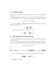
You will remember from your elementary physics courses 1 that if you want to know the<br />
electric field produced by a collection of point charges, you can figure this out by adding<br />
the field produced by each charge individually. That is, if we have n charges {q i } i=1,n<br />
,<br />
then the total electric field is (neglecting constant factors)<br />
E(q 1 + q 2 + · · · q n ) =<br />
n∑<br />
i=1<br />
q i<br />
(r − r i )<br />
|r − r i | 3 (1.0.1)<br />
where r is the observation point and r i is the position vector of the ith charge. The ith<br />
term in the sum on the right hand side,<br />
E(q i ) = q i<br />
(r − r i )<br />
|r − r i | 3 , (1.0.2)<br />
is the electric field of the ith point charge (Coulomb’s law). This property, whereby we<br />
can analyze a complicated system (in this case the total electric field E(q 1 +q 2 +· · · q n )) by<br />
breaking it into its constituent pieces (in this case E(q i )) and then adding up the results<br />
is known as linearity. There are three reasons why linear systems are so important.<br />
1. We can solve them. There are systematic mathematical techniques that let us<br />
tackle linear problems.<br />
2. Lots of physics is linear. Maxwell’s equations of electricity and magnetism for<br />
instance, or the elastic and acoustic wave equations.<br />
3. Lots of physics that is nonlinear is approximately linear at low energies or for small<br />
displacements from equilibrium.<br />
1
2 CHAPTER 1. SIMPLE HARMONIC MOTION: FROM SPRINGS TO WAVES<br />
θ<br />
Figure 1.1: A pendulum. The restoring force is the component of the gravitational force<br />
acting perpendicular to the wire supporting the mass. This is −mg sin(θ). Assuming the<br />
wire support is rigid, the acceleration of the mass is in the θ direction, so ma = ml¨θ and<br />
we have from Newton’s second law: ¨θ + g sin(θ) = 0. This is a nonlinear equation except<br />
l<br />
for small θ, in which case sin(θ) ≈ θ.<br />
m<br />
Here we introduce a nice, simplifying notation for derivatives of functions of time<br />
df(t)<br />
= f(t)<br />
dt<br />
˙ = f ˙<br />
d 2 f(t)<br />
=<br />
dt ¨f(t) = ¨f.<br />
2<br />
(1.0.3)<br />
For functions of some other variable we write<br />
dh(x)<br />
dx = h′ (x) = h ′<br />
d 2 h(x)<br />
dx 2 = h ′′ (x) = h ′′ .<br />
(1.0.4)<br />
For instance, the motion of a plane pendulum of length l (Figure 1.1) is governed by<br />
¨θ + g sin(θ) = 0. (1.0.5)<br />
l<br />
Equation 1.0.5 is not linear in θ. To solve it exactly we have to resort to elliptic functions<br />
or numerical methods. However, for small displacements (θ
1.1. A SPRING AND A MASS 3<br />
mately equal to θ. So for small displacements, the equation for the pendulum is<br />
¨θ + g θ = 0. (1.0.6)<br />
l<br />
Think of this equation as being the result of an operator acting on θ. Let’s call the<br />
operator L, in which case Equation 1.0.6 becomes L(θ) = 0. Why bother? Now we can<br />
see that<br />
L(θ 1 + θ 2 ) = d2 (θ 1 + θ 2 )<br />
+ g dt 2 l (θ 1 + θ 2 )<br />
( d 2 θ 1<br />
=<br />
dt + g ) ( d 2<br />
2 l θ θ 2<br />
1 +<br />
dt + g )<br />
2 l θ 2<br />
= L(θ 1 ) + L(θ 2 ). (1.0.7)<br />
A formal definition of a linear operator L, acting on numbers or vectors x and y is that<br />
L(ax + by) = aL(x) + aL(y) (1.0.8)<br />
for any a and b. Thus the equation of motion for the pendulum is linear in θ when θ is<br />
small.<br />
This is not an unusual situation. Suppose we have a point mass m constrained to move<br />
along the x-axis under the influence of some force F . Then Newton’s second law is<br />
mẍ = F (x). Suppose x 0 is an equilibrium point of the system, so F (x 0 ) = 0. Then<br />
expanding F in a Taylor series about x 0 we have<br />
mẍ = F ′ (x 0 )(x − x 0 ) + 1 2 F ′′ (x 0 )(x − x 0 ) 2 + · · · (1.0.9)<br />
If x is close to x 0 , then x − x 0 is small and we can drop all the terms past the first. 2<br />
If we do drop the higher order terms, Equation 1.0.9 becomes linear in x − x 0 . Since<br />
we said nothing at all about F itself, only that x is close to an equilibrium position,<br />
this argument applies to any F and is therefore one reason that nature appears linear so<br />
much of the time.
4 CHAPTER 1. SIMPLE HARMONIC MOTION: FROM SPRINGS TO WAVES<br />
k<br />
k<br />
Equilibrium<br />
x<br />
Figure 1.2: A linear spring satisfies Hooke’s law: the force applied by the spring to a mass<br />
is proportional to the displacement of the mass from its equilibrium, with the proportionality<br />
being the spring constant. Since the spring wants to return to its equilibrium,<br />
the force must have the opposite sign as the displacement. Thus mass times acceleration<br />
mẍ = −kx.<br />
1.1 A Spring and a Mass<br />
1.1.1 Simple harmonic oscillation<br />
Figure 1.2 shows a mass suspended from a spring. On the left, the mass and spring are in<br />
equilibrium. On the right the system has been displaced a distance x from equilibrium. 3<br />
The spring is said to be linear if it satisfies Hooke’s law: the force applied to the mass is<br />
proportional to its displacement from equilibrium.<br />
Robert Hooke (Born: July 1635, Isle of Wight, Died: March 1703 in London) was<br />
an English natural scientist. He first published his law in 1676 as a Latin anagram:<br />
ceiiinosssttuv. Three years later he published the solution: ut tensio sic vis, more or<br />
less “as the force, so the displacement”. Hooke attempted to prove that the Earth<br />
moves in an ellipse round the Sun and conjectured an inverse square law for gravity.<br />
Unfortunately, no portrait of Hooke is known to exist.<br />
The constant of proportionality is called the spring constant and is usually denoted by<br />
k. Since the force wants to restore the mass to its equilibrium, it must have the opposite<br />
2 This is an example of a common sort of approximation. Unless x = x 0 all the powers appearing<br />
in the Taylor series are potentially nonzero, but their importance decreases with increasing power; the<br />
most important being the lowest or leading order. In this case the leading order term is x − x 0 . If<br />
x − x 0 is .1 for instance, then by dropping terms beyond the first we are introducing an error of order<br />
.01. Conversely, if we want to achieve an accuracy of a given order, then we can work out how many<br />
terms in the Taylor series are needed to achieve that accuracy.<br />
3 In the next section we will take gravity into account.
1.1. A SPRING AND A MASS 5<br />
sign of the displacement. Thus mass times acceleration mẍ = −kx:<br />
Hooke’s Law mẍ = F = −kx. (1.1.1)<br />
Equation 1.1.1 is a simple example of a linear, constant coefficient, ordinary differential<br />
equation. You learned how to solve this equation by mathematics in your differential<br />
equations class. Here we think about the physics. Since Equation 1.1.1 is supposed to<br />
model the motion of the spring/mass system, let’s see experimentally what that motion<br />
really is. I went to the hardware store and bought a spring of unknown properties and<br />
attached a 375 g mass to the end. Pull the mass down a little bit and let it go. Now<br />
count the number of complete oscillations in, say, 15 seconds. For this spring we get 19<br />
complete oscillations. That’s just under 1.3 oscillations per second, or 1.3 Hz.<br />
Now pull the mass down twice as far and let it go. Count the oscillations. We still<br />
get 19. This is an interesting fact: the frequency of oscillation is independent of<br />
the amplitude of the motion. That means that the solution of Equation 1.1.1 must<br />
be a function that is periodic, with a fixed period of 1/1.3, since every 1/1.3 seconds<br />
the motion repeats. So x(t) = cos(ωt) or x(t) = sin(ωt) where ω = 2π 1.3 radians per<br />
second. 4<br />
Hz is Short for Hertz, after the German physicist Heinrich Hertz.<br />
Hertz was born in Hamburg in 1857 and studied at the University<br />
of Berlin. Hertz is best known as the first to broadcast and receive<br />
radio waves: a profoundly influential discovery. Less well known is the<br />
fact that Hertz also discovered the photoelectric effect, while pursuing<br />
his research into radio waves. A modest man, Hertz died at the age<br />
of 37 in 1894 from blood poisoning. His brief career as a professor was spent at the<br />
Universities of Karlsruhe and Bonn.<br />
Since there is no absolute scale of time, we are free to choose the origin of the time axis<br />
however we wish. In this experiment it seems reasonable to choose the point t = 0 to<br />
correspond to the time we let the mass go. That being the case, the solution must be<br />
x(t) = A cos(ωt) since sin(0) = 0. Now x(0) = A so the constant A corresponds to the<br />
amplitude of displacement. If we plug x(t) = A cos(ωt) into Equation 1.1.1, then this<br />
is indeed a solution for any A provided that ω 2 = k/m. This makes sense qualitatively,<br />
since increasing the mass should decrease the frequency: the greater mass stretches the<br />
spring more and so takes longer to complete each oscillation. On the other hand, if we<br />
increase k we are making the spring stiffer, so it oscillates faster.<br />
But let’s see if this analysis holds up experimentally. Let’s increase the mass a little<br />
bit by adding a 60 g magnet to it. Count the oscillations again. This time we get only<br />
4 Frequencies in Hz are usually denoted by an f. ω is almost universally used for circular frequencies.<br />
Just remember that since the motion repeats itself once every 1/f seconds, the argument of the sine<br />
function must increase by 2π during this time.
6 CHAPTER 1. SIMPLE HARMONIC MOTION: FROM SPRINGS TO WAVES<br />
18 oscillations in 15 seconds, or 1.2 Hz. So by increasing the mass by about 16% we’ve<br />
decreased the frequency of oscillation by about 8%. That means the frequency must go<br />
as one over the square root of the mass! Not convinced? We can use a Taylor series to<br />
do a perturbation analysis (using m 0 to denote the unperturbed mass):<br />
ω(m) ≈ ω(m 0 ) + ω ′ (m 0 )δm<br />
= ω 0 − 1 2<br />
√<br />
k<br />
m 3 0<br />
δm defining ω 0 = ω(m 0 )<br />
= ω 0 − 1 √<br />
2 ω δm<br />
k<br />
0 since ω 0 =<br />
m 0 m 0<br />
= ω 0 (1 − 1 δm<br />
)<br />
2 m 0<br />
= 2π 1.3(1 − 1 60<br />
) = 2π 1.3 × .92 ≈ 2π 1.2r/s. (1.1.2)<br />
2 375<br />
So the theory holds water. NB. The argument of the sinusoid is an angle. Therefore<br />
during one complete oscillation, the angle goes through 2π radians.<br />
No matter<br />
√<br />
how we start the spring/mass system going, it always oscillates with the<br />
frequency k<br />
. So this is its natural or characteristic frequency. Let’s continue to<br />
m<br />
refer to this characteristic frequency as ω 0 to emphasize the fact that it is a constant for<br />
a given spring/mass system.<br />
Exercise on spring constants<br />
First compute the spring constant of the spring using the data above. You’ll see that<br />
with or without the added 60 g mass, the spring constant is about 25 N/m. Now<br />
consider the “spring constant” of a diatomic molecule. Look up the mass of a nitrogen<br />
or oxygen molecule, for example. You can assume that the resonant frequency is in<br />
the infrared (why?), which makes it about 10 13 Hz. What you will find is that the<br />
spring constant is within a factor of 2 or 3 the same as the spring we used in class!<br />
Spring/mass or spring + mass?<br />
Scenario 1: We suspend the spring without a mass. It has some relaxed length l. Now<br />
attach the mass m. It stretches the spring a little bit ∆l. This stretching is caused by the<br />
weight (gravitational force) of the mass: mg. So mg = k∆l. (Since in equilibrium the<br />
total force is zero: mg + (−k∆l) = 0.) Now pull the mass down a little bit and let it go.<br />
The total displacement from the equilibrium position of the spring alone is ∆l + x. So<br />
the restoring force of the spring is −k(∆l + x). Thus the total force on the mass (spring<br />
+ gravity, but no damping for now) is mg − k(∆l + x). But since mg = k∆l, this reduces<br />
to −kx. Thus, even if we explicitly include gravity and the original relaxed length of
1.1. A SPRING AND A MASS 7<br />
k<br />
k<br />
relaxed length<br />
spring/mass equilibrium<br />
x<br />
Figure 1.3: The relaxed length of the spring with no mass attached (left). Adding the<br />
mass increases the relaxed length but does not change the motion, provided the spring<br />
is linear.<br />
the spring, we end up with mẍ + kx = 0 as the equations of motion. This is shown in<br />
Figure 1.3.<br />
As an aside, the fact that mg = k∆l gives us a connection between g and ω 0 : g/∆l = ω0.<br />
2<br />
For the spring we used above ∆l was about 9 cm. The frequency is √ 980<br />
/2π ≈ 1.7. This<br />
9<br />
is a bit higher than measured, but our theory is approximate since we’ve neglected the<br />
finite mass of the spring itself.<br />
Scenario 2: We suspend the spring with the mass and take the relaxed position of the<br />
combined spring/mass system as the equilibrium state and measure displacements from<br />
this position. Ignoring gravity, we still get mẍ + kx = 0. In effect what we’ve done is to<br />
use the mass m to increase the relaxed length of the spring. Since the spring is linear, a<br />
constant change in the equilibrium position has no effect on the motion.<br />
Sine or Cosine?<br />
At first glance it seems odd that something as arbitrary as the choice of the origin of time<br />
could influence our solution. Once the mass is oscillating we could just as easily suppose<br />
that the time at which it passes through the origin is t = 0. But then the “initial”<br />
displacement would be zero (since the mass is at the origin), while the initial velocity<br />
would be non-zero. That would make the displacement proportional to a sine function,<br />
say x(t) = B sin(ω 0 t). Then x(0) = 0 and ẋ(0) = ω 0 B. So B must equal whatever<br />
velocity the mass has when it zips through the origin, divided by the characteristic<br />
frequency ω 0 . So it looks like we can have either<br />
taking t = 0 as the time at which we let the mass go, or<br />
x(t) = x(0) cos(ω 0 t), (1.1.3)<br />
x(t) = ẋ(0)<br />
ω 0<br />
sin(ω 0 t), (1.1.4)
8 CHAPTER 1. SIMPLE HARMONIC MOTION: FROM SPRINGS TO WAVES<br />
taking t = 0 as the time at which the spring passes through the origin with velocity ẋ(0).<br />
Mathematically this amounts to saying that we must specify both x(0) and ẋ(0) since<br />
the equations of motion are second order. Physically this amounts to noticing that the<br />
motion is the same no matter how we choose the origin of time. We can cover all the<br />
bases by writing the displacement as<br />
x(t) = A cos(ω 0 (t + t 0 )) = A cos(ω 0 t + ∆) (1.1.5)<br />
where t 0 is an arbitrary time shift. It’s a little cleaner if we absorb the product of ω 0 and<br />
t 0 as a single, dimensionless phase constant ∆. Using the law of addition of cosines, this<br />
last expression can be written<br />
x(t) = A cos(ω 0 t + ∆) = A cos(ω 0 t) cos(∆) − A sin(ω 0 t) sin(∆)<br />
= a cos(ω 0 t) + b sin(ω 0 t), (1.1.6)<br />
where a = A cos(∆) and b = −A sin(∆). No matter how we write it, we must specify two<br />
constants: x(0), ẋ(0); A, t 0 ; A, ∆; a, b.<br />
Energy is conserved<br />
So far we have not accounted for the damping of the spring. Theoretically, once started<br />
in motion it should oscillate at ω 0 Hz forever. Later we will take into account the<br />
actual dissipation of energy in the spring, but for now as a check we should verify that<br />
the solution we have obtained really does conserve energy. The total energy of the<br />
spring/mass system is a combination of the kinetic energy of the mass 1/2mẋ 2 and the<br />
potential energy of the spring. The force −kx is minus the derivative of 1/2kx 2 , so this<br />
must be the potential energy. It is generally true that if energy is conserved, the force is<br />
minus the gradient (d/dx in the one-dimensional case) of a potential energy function.<br />
OK, so the total energy of the spring/mass system is the sum of the kinetic and potential<br />
energies:<br />
Using the general solution x(t) = A cos(ω 0 t + ∆) we have<br />
E = T + U = 1 2 mẋ2 + 1 2 kx2 . (1.1.7)<br />
E = 1 2 mω2 0 A2 sin 2 (ω 0 t + ∆) + 1 2 kA2 cos 2 (ω 0 t + ∆)<br />
= 1 2 kA2 sin 2 (ω 0 t + ∆) + 1 2 kA2 cos 2 (ω 0 t + ∆)<br />
= kA 2 . (1.1.8)<br />
Since the t disappears, we see that the energy is constant with time, and thus energy is<br />
conserved. The reasoning is somewhat circular however, since we can’t really take the<br />
force to be the gradient of a potential unless energy is conserved.
1.1. A SPRING AND A MASS 9<br />
1.1.2 Forced motion<br />
When the mass shown in Figure 1.2 is bouncing up and down, we can tap it gently<br />
from below. Notice that if you tap it at just the natural frequency ω 0 , your taps are<br />
synchronized with the motion, so the energy you apply goes directly into increasing the<br />
amplitude of the oscillation. The same thing happens when you’re swinging in a swing.<br />
If you swing your legs back and forth with the natural frequency of the swing, you’ll get<br />
a big amplification of your motion. This is called a resonance. To model it we need to<br />
add another term to the equation of motion of the spring/mass.<br />
mẍ(t) + kx(t) = F (t). (1.1.9)<br />
Because the motion of the mass is oscillatory, the easiest sorts of forces to deal with<br />
will be oscillatory too. Later we will see that it is no loss to treat sinusoidal forces; the<br />
linearity of the equations will let us build up the result for arbitrary forces by adding a<br />
bunch of sinusoids together. But for now, let’s just suppose that the applied force has<br />
the same form as the unforced motion of the mass:<br />
mẍ(t) + kx(t) = F 0 cos(ωt). (1.1.10)<br />
The forcing function doesn’t know anything about the natural frequency of the system<br />
and there is no reason why the forced oscillation of the mass will occur at ω 0 . Of course,<br />
we will be especially interested in the solution when ω = ω 0 . To keep the algebra simple,<br />
let’s take the phase ∆ equal to zero and look for solutions of the form<br />
Plugging this into Equation 1.1.10 we have<br />
x(t) = A cos(ωt). (1.1.11)<br />
(−ω 2 + ω0 2 )A cos(ωt) = F 0<br />
cos(ωt). (1.1.12)<br />
m<br />
The cosines cancel and we are left with an equation for the amplitude of motion:<br />
A = F 0 1<br />
m ω0 2 − ω . (1.1.13)<br />
2<br />
Notice especially what happens if we force the system at the natural frequency: ω = ω 0<br />
and the amplitude blows up. In practice the amplitude never becomes infinite. In the<br />
first place the spring would stretch to the point of breaking; but also, dissipation, which<br />
we have neglected, would come into play. Nevertheless, the idea is sound. If we apply a<br />
force to a system at its characteristic frequency we should expect a big effect.<br />
Forced and free oscillations<br />
The motion of the mass with no applied force is an example of a free oscillation. Otherwise<br />
the oscillations are forced. An important example of a free oscillation is the motion
10 CHAPTER 1. SIMPLE HARMONIC MOTION: FROM SPRINGS TO WAVES<br />
of the entire earth after a great earthquake. Free oscillations are also called transients<br />
since for any real system in the absence of a forcing term, the damping will cause the<br />
motion to die out<br />
1.1.3 Complex numbers and constant coefficient differential<br />
equations<br />
We solved the equations of the simple spring/mass system ẍ(t) + ω0 2 x = 0 by thinking<br />
about the physics. This is an example of a constant coefficient differential equation.<br />
The coefficients are the terms multiplying the derivatives of the independent variable.<br />
(x is the zeroth derivative of x.) The most general linear nth order constant coefficient<br />
differential equation is<br />
d n x<br />
a n<br />
dt + a d n−1 x<br />
n n−1<br />
dt + · · · a dx<br />
n−1 1<br />
dt + a 0x = 0. (1.1.14)<br />
These constant coefficient differential equations have a very special property: they reduce<br />
to polynomials for exponential x. To see this, plug an exponential e pt into Equation 1.1.14.<br />
The ith derivative with respect to time is p i e pt , so Equation 1.1.14 becomes<br />
(<br />
an p n + a n−1 p n−1 + · · · + a 1 p + a 0<br />
)<br />
e pt = 0. (1.1.15)<br />
Canceling the overall factor of e pt we see that solving Equation 1.1.14 reduces to finding<br />
the roots of an nth order polynomial. For n = 2, we know the formula for the roots<br />
p = −a 1 ±<br />
√<br />
a 2 1 − 4a 0 a 2<br />
2a 2<br />
. (1.1.16)<br />
When n is greater than 2 life becomes more complicated; fortunately most equations in<br />
physics are first or second order.<br />
For example, suppose<br />
ẍ + x = 0, (1.1.17)<br />
so a 2 = 1, a 1 = 0, and a 0 = 1. Then p = ± √ −1. √ −1 = i is called the pure imaginary<br />
number. Here we see the main reason for complex numbers. Without i, not even a simple<br />
equation such as ẍ+x = 0 has a solution. With i every algebraic equation can be solved.<br />
Complex numbers are things of the form a+ib where a and b are real numbers. We can<br />
think of 1 and i as being basis vectors in a two-dimensional Cartesian space. Addition of<br />
complex numbers is component-wise: (a+ib)+(p+iq) = (a+p)+i(b+q). Multiplication<br />
is as you would expect, but with ii = −1. So (a + ib)(p + iq) = (ab − bq) + i(bp + aq).<br />
In the complex plane, multiplication by i acts as a rotation by π/4. i1 = i, ii = −1,<br />
i(−1) = −i and i(−i) = 1. (Figure 1.4.)
1.1. A SPRING AND A MASS 11<br />
1 i = i*1<br />
-1 = i*i -i = i*(-1)<br />
Figure 1.4: Multiplication by the pure imaginary i acts as a π/4 rotation in the complex<br />
plane.<br />
And just as there is an equivalence between Cartesian and polar coordinates, so we can<br />
give a “polar” representation of every complex number. To understand this connection,<br />
consider the Maclauren series for e x<br />
Now replace x with ix. We get<br />
e x = 1 + x + x2<br />
2 + x3<br />
6 + x4<br />
24 + x5<br />
120 + x6<br />
720 + · · · (1.1.18)<br />
e ix = 1 + ix + (ix)2<br />
[ 2<br />
=<br />
+ (ix)3<br />
6<br />
1 − x2<br />
2 + x4<br />
24 + · · ·]<br />
+ i<br />
+ (ix)4<br />
24 + (ix)5<br />
120 + (ix)6<br />
720 + · · ·<br />
[<br />
·]<br />
x − x3<br />
6 + x5<br />
120 + · ·<br />
(1.1.19)<br />
In the limit of small x, this reduces to e ix ≈ 1 + ix, which is the small angle limit of<br />
cos(x) + i sin(x). To see if this extends to large x, compute the Maclauren series for the<br />
sine and cosine:<br />
cos(x) = 1 − x2<br />
2 + x4<br />
24 + · · · (1.1.20)<br />
sin(x) = x − x3<br />
6 + x5<br />
120 + · · · . (1.1.21)<br />
Thus we have proved what some call the most remarkable formula in mathematics:<br />
Euler’s Formula e ix = cos(x) + i sin(x). (1.1.22)<br />
The geometry of the Cartesian and polar representations is summarized in Figure 1.5.
12 CHAPTER 1. SIMPLE HARMONIC MOTION: FROM SPRINGS TO WAVES<br />
imaginary axis<br />
z<br />
r<br />
y<br />
θ<br />
x<br />
real axis<br />
Figure 1.5: Every complex number z can be represented as a point in the complex plain.<br />
There are various ways or “coordinates” by which we can parameterize these points.<br />
The Cartesian parameterization is in terms of the real and imaginary parts. The polar<br />
parameterization is in terms of the length (or modulus) and angle (or phase). The<br />
connection between these two forms is the remarkable Euler formula: re iθ = r cos θ +<br />
ir sin θ. From Pythagoras’ theorem we can see r 2 = x 2 + y 2 and the angle θ is just the<br />
arctangent of y/x.<br />
1.1.4 Forced motion with damping<br />
Now let’s go ahead and do the fully general simple harmonic oscillator, including the<br />
effects of damping (i.e., dissipations). The causes of damping are extremely subtle. We<br />
will not go deeply into these effects here except to say that ultimately the physical processes<br />
which cause damping give rise to motion at the atomic and molecular level. If you<br />
calculate the characteristic frequencies of atoms, as we have done for the spring/mass<br />
system, you see that these frequencies are the same as electromagnetic radiation in the<br />
infrared. Heat in other words! But this heat is just the manifestation of a kind of oscillatory<br />
motion. When the energy of these oscillations is not too great, the atoms/molecules<br />
can be treated as simple harmonic oscillators.<br />
However, it has long been observed empirically that to a reasonable approximation, the<br />
effect of damping or friction is to oppose the motion of the mass with a force that is<br />
proportional to the velocity. If the mass is at rest, there is no friction. As the velocity<br />
increases, the frictional force increases and this force opposes the motion. Try extending<br />
a damping piston of the sort used on doors. The faster you extend the piston, the greater<br />
the resistance. So as a first approximation, we can model the friction of our spring/mass<br />
system as<br />
ẍ + γẋ + ω 2 0 x = F m<br />
(1.1.23)<br />
where γ is a constant reflecting the strength of the damping. We can proceed just as<br />
before with the undamped, forced oscillations but the algebra is greatly simplified if we
1.1. A SPRING AND A MASS 13<br />
use complex numbers. We have used cos(ωt) to represent a oscillatory driving force.<br />
From Euler’s formula we know that the cosine is the real part of e iωt . So we are going to<br />
use a trick. We are going to use e iωt throughout the calculation and then take the real<br />
part when we’re done. The reason for doing this is simply that exponentials are easier<br />
to work with than cosines. The fact that we get the right answer in the end depends<br />
critically on the equations being linear. This trick will not work for nonlinear equations.<br />
To prove this to yourself, assume for the moment that x = x r + ix i and F = F r + iF i .<br />
Plug these into Equation 1.1.23 and show that<br />
ẍ r + γx˙<br />
r + ω0x 2 r + i [ ]<br />
ẍ i + γx˙<br />
i + ω0x 2 F r<br />
i =<br />
m + iF i<br />
m . (1.1.24)<br />
In order for two complex numbers to be equal, their real and imaginary parts must be<br />
equal separately. Therefore the real part of the complex “displacement” must satisfy<br />
Equation 1.1.23, which is what was claimed.<br />
So let’s write the complex force as F = ˆF e iωt and the complex displacement as x = ˆxe iωt .<br />
Plugging this into Equation 1.1.23 implies that<br />
Canceling the exponential gives<br />
(−ω 2 + iγω + ω 2 0)ˆxe iωt = ˆF<br />
m eiωt . (1.1.25)<br />
ˆx =<br />
ˆF /m<br />
. (1.1.26)<br />
−ω 2 + iγω + ω0<br />
2<br />
This equation requires a little analysis, but straight off we can see that the presence of<br />
the damping term γ has fixed the infinity we saw when we forced the oscillator at its<br />
resonant frequency; even when ω = ω 0 the amplitude is finite provided γ is not zero. For<br />
the moment let’s just look at the denominator of the displacement.<br />
−ω 2 + iγω + ω 2 0 =<br />
γω<br />
√(ω0 2 − ω 2 ) 2 + γ 2 ω 2 i tan−1<br />
ω<br />
e 0 2−ω2 . (1.1.27)<br />
The function ρ 2 = 1/((ω 2 0 − ω2 ) 2 + γ 2 ω 2 ) has a characteristic shape seen in all resonance<br />
phenomena. It’s peaked about the characteristic frequency ω 0 and has a full width of γ<br />
at half its maximum height as illustrated in Figure 1.6.<br />
Finally, since γ has the dimension of inverse time, a useful dimensionless measure of<br />
damping can be obtained by taking the ratio of the characteristic frequency ω 0 and<br />
γ. This ratio is called the Q (for quality factor) of the peak. Typical values of Q at<br />
ultrasonic frequencies can range from 10-100 for sedimentary rocks, to a few thousand<br />
for aluminum, to nearly a million for monocrystalline quartz.
14 CHAPTER 1. SIMPLE HARMONIC MOTION: FROM SPRINGS TO WAVES<br />
ρ<br />
γ<br />
ω 0<br />
ω<br />
Figure 1.6: Square of the amplitude factor ρ 2 = 1/((ω 2 0 −ω 2 ) 2 +γ 2 ω 2 ) for forced, damped<br />
motion near a resonance ω 0 . The full width at half max of this curve is the damping<br />
factor γ, provided γ is small!<br />
1.5<br />
arctangent<br />
1<br />
0.5<br />
0<br />
−0.5<br />
−1<br />
−1.5<br />
−10 −5 0 5 10<br />
Figure 1.7: The arctangent function asymptotes at ±π/2, so we should expect to see a<br />
phase shift of π when going through a resonance.
1.1. A SPRING AND A MASS 15<br />
RMS amplitude<br />
0.030<br />
0.020<br />
0.010<br />
0.020<br />
0.010<br />
0.000<br />
48.0 48.4 48.8<br />
0.000<br />
0 50 100 150 200<br />
frequency (kHz)<br />
Figure 1.8: Here is a resonance spectrum for a piece of aluminum about the size shown in<br />
Figure 1.9. A swept sine wave is fed into the sample via a tiny transducer and recorded<br />
on another transducer. At a resonant frequency, there is a big jump in the amplitude.<br />
The DC level is shifted upward to make it easy to see the peaks. The inset shows a<br />
blow-up of one peak.<br />
Figure 1.9: Resonance ultrasonic spectroscopy setup. The rock is held fast by two tiny<br />
transducers (“pinducers”) which are used to transmit a signal and record the response.<br />
The two traces shown on the oscilloscope correspond to the transmitted and received<br />
signal. As the frequency is varied we see the characteristic resonance (cf Figure 1.8). To<br />
a first approximation, the frequency associated with the peak is one of the characteristic<br />
(eigen) frequencies of the sample.
16 CHAPTER 1. SIMPLE HARMONIC MOTION: FROM SPRINGS TO WAVES<br />
1.1.5 Damped transient motion<br />
Suppose we suspend our mass in a viscous fluid. Pull it down and let it go. The fluid will<br />
damp out the motion, more or less depending on whether it has the viscosity of water or<br />
honey. Mathematically this case is easy, all we have to do is set the right hand side of<br />
Equation 1.1.25 to zero. This leaves a simple quadratic for ω<br />
which has the two solutions<br />
ω 2 − iγω − ω 2 0 = 0 (1.1.28)<br />
√<br />
ω = iγ ± 4ω0 2 − γ 2<br />
2<br />
= i γ √<br />
( ) γ 2.<br />
2 ± ω 0 1 −<br />
(1.1.29)<br />
2ω 0<br />
These give the following solutions for the motion (using x(0) = x 0 )<br />
√<br />
(<br />
x(t) = x 0 e − γ 2 t e ±itω 0<br />
1−<br />
γ<br />
2ω 0<br />
) 2<br />
. (1.1.30)<br />
This looks like the equation of a damped sinusoid. But the second term may or may not<br />
be a sinusoid, depending on whether the square root is positive. So we have to treat two<br />
γ<br />
special cases. First if<br />
2ω 0<br />
< 1, corresponding to small damping, then the argument of<br />
the square root is positive and indeed we have a damped sinusoid. On the other hand if<br />
> 1, then we can rewrite the solution as<br />
γ<br />
2ω 0<br />
x(t) = x 0 e − γ 2 t e ±tω 0<br />
√<br />
( γ<br />
2ω 0<br />
) 2 −1<br />
(1.1.31)<br />
where, once again, we have arranged things so that the argument of the square root is<br />
positive. But now only the minus sign in the exponent makes sense, since otherwise the<br />
amplitude of the motion would increase with time. So, we have<br />
√<br />
x(t) = x 0 e − γ 2 t e −ω 0t ( γ ) 2ω 2 −1 0 . (1.1.32)<br />
In this case the motion is said to be “over-damped” since there is no oscillation. In a<br />
highly viscous fluid (high relative to ω 0 ) there is no oscillation at all, the motion is quickly<br />
damped to zero. The borderline case γ = 2ω 0 is called critical damping, in which case<br />
x(t) = x 0 e − γ 2 t .<br />
1.1.6 Another velocity-dependent force: the Zeeman effect<br />
As a classical model for the radiation of light from excited atoms we can consider the<br />
electrons executing simple harmonic oscillations about their equilibrium positions under
1.1. A SPRING AND A MASS 17<br />
the influence of a restoring force F = −kr. Thus our picture is of an oscillating electric<br />
dipole. Remember, the restoring force −kr is just a linear approximation to the Coulomb<br />
force and therefore k, the “spring constant”, is the first derivative of the Coulomb force<br />
evaluated at the equilibrium radius of the electron. So the vector differential equation<br />
governing this simple harmonic motion is:<br />
m¨r + kr = 0. (1.1.33)<br />
Notice that there is no coupling between the different components of r. In other words<br />
this one vector equation is equivalent to three completely separate scalar equations (using<br />
ω 2 0 = k/m)<br />
ẍ + ω 2 0 x = 0<br />
ÿ + ω 2 0y = 0<br />
¨z + ω 2 0 z = 0<br />
each of which has the same solution, a sinusoidal oscillation at frequency ω 0 . Think of<br />
it this way: there are three equations and three frequencies of oscillation, but all the<br />
frequencies happen to be equal. This is called degeneracy. The equations are uncoupled<br />
in the sense that each unknown (x, y, z) occurs in only one equation; thus we can solve<br />
for x ignoring y and z.<br />
Now let’s suppose we apply a force that is not spherically symmetric. For instance,<br />
suppose we put the gas of atoms in a magnetic field pointed along, say, the z-axis. This<br />
results in another force on the electrons of the form qṙ × Bẑ (from Lorentz’s force law).<br />
Adding this force to the harmonic (−kr) force gives 5<br />
ẍ + ω 2 0x − qB m ẏ = 0<br />
ÿ + ω 2 0y + qB m ẋ = 0<br />
¨z + ω 2 0 z = 0.<br />
The z equation hasn’t changed so it’s still true that z(t) = Real(z 0 e iω 0t ). But now the x<br />
and y equations are coupled–we must solve for x and y simultaneously. Let us assume a<br />
solution of the form:<br />
x(t) = Real(x 0 e iωt )<br />
y(t) = Real(y 0 e iωt )<br />
5 Remember the right-hand screw rule, so ŷ × ẑ = ˆx, ˆx × ẑ = −ŷ, and ẑ × ẑ = 0
18 CHAPTER 1. SIMPLE HARMONIC MOTION: FROM SPRINGS TO WAVES<br />
where x 0 and y 0 are constants to be determined. Plugging these into the equations for x<br />
and y gives the two amplitude equations<br />
(ω 2 0 − ω2 )x 0 = qB m iωy 0 (1.1.34)<br />
(ω 2 0 − ω2 )y 0 = − qB m iωx 0.<br />
We can use the first equation to compute x 0 in terms of y 0 and then plug this into the<br />
second equation to get<br />
( qB<br />
(ω0 2 − ω 2 m<br />
)y 0 = −<br />
iω) 2<br />
ω0 2 − ω y 0.<br />
2<br />
Now we eliminate the y 0 altogether and get<br />
(<br />
ω<br />
2<br />
0 − ω 2) 2<br />
=<br />
( qB<br />
m ω ) 2<br />
(1.1.35)<br />
Taking the square root we have<br />
ω0 2 − ω 2 = ± qB ω. (1.1.36)<br />
m<br />
This is a quadratic equation for the unknown frequency of motion ω. So we have<br />
√ (<br />
ω = ± qB ± qB<br />
m m<br />
2<br />
) 2<br />
+ 4ω<br />
2<br />
0<br />
. (1.1.37)<br />
This is not too bad, but we can make a great simplification by assuming that the magnetic<br />
field is weak. Specifically, let’s assume that qB m
1.2. TWO COUPLED MASSES 19<br />
m1<br />
m2<br />
k1 k2 k3<br />
Figure 1.10: Two masses coupled by a spring and attached to walls.<br />
This splitting of the degenerate frequency by an external magnetic<br />
field is called the Zeeman effect, after its discoverer Pieter Zeeman<br />
was born in May 1865, at Zonnemaire, a small village in the isle of<br />
Schouwen, Zeeland, The Netherlands. Zeeman was a student of the<br />
great physicists Onnes and Lorentz in Leyden. He was awarded the<br />
Nobel Prize in Physics in 1902. Zeeman succeeded Van der Waals<br />
(another Nobel prize winner) as professor and director of the Physics Laboratory in<br />
Amsterdam in 1908. In 1923 a new laboratory was built for Zeeman that included a<br />
quarter-million kilogram block of concrete for vibration free measurements.<br />
We could continue the analysis by plugging these frequencies back into the amplitude<br />
equations 1.1.35. As an exercise, do this and show that the motion of the electron<br />
(and hence the electric field) is circularly polarized in the direction perpendicular to the<br />
magnetic field.<br />
1.2 Two Coupled Masses<br />
With only one mass and one spring, the range of motion is somewhat limited. There is<br />
only one characteristic frequency ω0 2 = k so in the absence of damping, the transient<br />
m<br />
(unforced) motions are all of the form cos(ω 0 t + ∆).<br />
Now let us consider a slightly more general kind of oscillatory motion. Figure 1.10 shows<br />
two masses (m 1 and m 2 ) connected to fixed walls with springs k 1 and k 3 and connected<br />
to one another by a spring k 2 . To derive the equations of motion, let’s focus attention<br />
on one mass at a time. We know that for any given mass, say m i (whose displacement<br />
from equilibrium we label x i ) it must be that<br />
m i ẍ i = F i (1.2.1)<br />
where F i is the total force acting on the ith mass. No matter how many springs and<br />
masses we have in the system, the force applied to a given mass must be transmitted<br />
by the two springs it is connected to. And the force each of these springs transmits is<br />
governed by the extent to which the spring is compressed or extended.
20 CHAPTER 1. SIMPLE HARMONIC MOTION: FROM SPRINGS TO WAVES<br />
Referring to Figure 1.10, spring 1 can only be compressed or extended if mass 1 is<br />
displaced from its equilibrium. Therefore the force applied to m 1 from k 1 must be −k 1 x 1 ,<br />
just as before. Now, spring 2 is compressed or stretched depending on whether x 1 − x 2<br />
is positive or not. For instance, suppose both masses are displaced to the right (positive<br />
x i ) with mass 1 being displaced more than mass 2. Then spring 2 is compressed relative<br />
to its equilibrium length and the force on mass 1 will in the negative x direction so as to<br />
restore the mass to its equilibrium position. Similarly, suppose both masses are displaced<br />
to the right, but now with mass 2 displaced more than mass 1, corresponding to spring 2<br />
being stretched. This should result in a force on mass 1 in the positive x direction since<br />
the mass is being pulled away from its equilibrium position. So the proper expression of<br />
Hooke’s law in any case is<br />
m 1 ẍ 1 = −k 1 x 1 − k 2 (x 1 − x 2 ). (1.2.2)<br />
And similarly for mass 2<br />
m 2 ẍ 2 = −k 3 x 2 − k 2 (x 2 − x 1 ). (1.2.3)<br />
These are the general equations of motion for a two mass/three spring system. Let us<br />
simplify the calculations by assuming that both masses and all three springs are the<br />
same. Then we have<br />
and<br />
ẍ 1 = − k m x 1 − k m (x 1 − x 2 )<br />
= −ω 2 0x 1 − ω 2 0(x 1 − x 2 )<br />
= −2ω 2 0 x 1 + ω 2 0 x 2. (1.2.4)<br />
ẍ 2 = − k m x 2 − k m (x 2 − x 1 )<br />
= −ω 2 0 x 2 − ω 2 0 (x 2 − x 1 )<br />
= −2ω 2 0x 2 + ω 2 0x 1 . (1.2.5)<br />
Assuming trial solutions of the form<br />
we see that<br />
Substituting one into the other we get<br />
x 1 = Ae iωt (1.2.6)<br />
x 2 = Be iωt (1.2.7)<br />
(−ω 2 + 2ω 2 0 )A = ω2 0 B (1.2.8)<br />
(−ω 2 + 2ω 2 0)B = ω 2 0A. (1.2.9)<br />
A =<br />
ω0<br />
2 B, (1.2.10)<br />
2ω0 2 − ω2
1.2. TWO COUPLED MASSES 21<br />
and therefore<br />
(2ω 2 0 − ω 2 )B =<br />
ω0<br />
4 B. (1.2.11)<br />
2ω0 2 − ω2 This gives an equation for ω 2 (2ω 2 0 − ω2 ) 2 = ω 4 0 . (1.2.12)<br />
There are two solutions of this equation, corresponding to ±ω0 2<br />
root. If we choose the plus sign, then<br />
when we take the square<br />
On the other hand, if we choose the minus sign, then<br />
2ω 2 0 − ω2 = ω 2 0 ⇒ ω2 = ω 2 0 . (1.2.13)<br />
2ω 2 0 − ω 2 = −ω 2 0 ⇒ ω 2 = 3ω 2 0. (1.2.14)<br />
We have discovered an important fact: spring systems with two masses have two characteristic<br />
frequencies. We will refer to the frequency ω 2 = 3ω 2 0 as “fast” and ω2 = ω 2 0<br />
as “slow”. Of course these are relative terms. Now that we have the frequencies we can<br />
investigate the amplitude. First, since<br />
we have for the slow mode (ω = ω 0 )<br />
A =<br />
ω0<br />
2 B, (1.2.15)<br />
2ω0 2 − ω2 A = B, (1.2.16)<br />
which corresponds to the two masses moving in phase with the same amplitude. On the<br />
other hand, for the fast mode<br />
A = −B. (1.2.17)<br />
For this mode, the amplitudes of the two mass’ oscillation are the same, but they are<br />
out of phase. These two motions are easy to picture. The slow mode corresponds to<br />
both masses moving together, back and forth, as in Figure 1.11 (bottom). The fast mode<br />
corresponds to the two masses oscillating out of phase as in Figure 1.11 (top).<br />
1.2.1 A Matrix Appears<br />
There is a nice way to simplify the notation of the previous section and to introduce a<br />
powerful mathematical at the same time. Let’s put the two displacements together into a<br />
vector. Define a vector u with two components, the displacements of the first and second<br />
mass:<br />
[ ] [ ]<br />
Ae<br />
iωt A<br />
u =<br />
Be iωt = e iωt . (1.2.18)<br />
B
22 CHAPTER 1. SIMPLE HARMONIC MOTION: FROM SPRINGS TO WAVES<br />
Figure 1.11: With two coupled masses there are two characteristic frequencies, one “slow”<br />
(bottom) and one “fast” (top).<br />
We’ve already seen that we can multiply any solution by a constant and still get a<br />
solution, so we might as well take A and B to be equal to 1. So for the slow mode we<br />
have<br />
[ ]<br />
u = e iω 0t 1<br />
, (1.2.19)<br />
1<br />
while for the fast mode we have<br />
u = e i√ 3ω 0 t<br />
[<br />
1<br />
−1<br />
]<br />
. (1.2.20)<br />
Notice that the amplitude part of the two modes<br />
[<br />
1<br />
1<br />
]<br />
and<br />
[<br />
1<br />
−1<br />
]<br />
(1.2.21)<br />
are orthogonal. That means that the dot product of the two vectors is zero: 1 × 1 +<br />
1 × (−1) = 0. 6 As we will see in our discussion of linear algebra, this means that the<br />
two vectors point at right angles to one another. This orthogonality is an absolutely<br />
fundamental property of the natural modes of vibration of linear mechanical systems.<br />
6<br />
[ 1<br />
1<br />
] [ 1<br />
·<br />
−1<br />
]<br />
[ 1<br />
≡ [1, 1]<br />
−1<br />
]<br />
= 1 · 1 − 1 · 1 = 0.
1.2. TWO COUPLED MASSES 23<br />
1.2.2 Matrices for two degrees of freedom<br />
The equations of motion are (see Figure 1.10):<br />
m 1 ẍ 1 + k 1 x 1 + k 2 (x 1 − x 2 ) = 0 (1.2.22)<br />
m 2 ẍ 2 + k 3 x 2 + k 2 (x 2 − x 1 ) = 0. (1.2.23)<br />
We can write these in matrix form as follows.<br />
[ ] [ ] [ ] [ ] [<br />
m1 0 ẍ1 k1 + k<br />
+<br />
2 −k 2 x1 0<br />
=<br />
0 m 2 ẍ 2 −k 2 k 2 + k 3 x 2 0<br />
Or, defining a mass matrix<br />
and a “stiffness” matrix<br />
K =<br />
we can write the matrix equation as<br />
M =<br />
[ ]<br />
m1 0<br />
0 m 2<br />
[ ]<br />
k1 + k 2 −k 2<br />
−k 2 k 2 + k 3<br />
]<br />
. (1.2.24)<br />
(1.2.25)<br />
(1.2.26)<br />
Mü + Ku = 0 (1.2.27)<br />
where<br />
[ ]<br />
x1<br />
u ≡ . (1.2.28)<br />
x 2<br />
This is much cleaner than writing out all the components and has the additional advantage<br />
that we can add more masses/springs without changing the equations, we just have<br />
to incorporate the additional terms into the definition of M and K.<br />
Notice that the mass matrix is always invertible since it’s diagonal and all the masses<br />
are presumably nonzero. Therefore<br />
M −1 =<br />
[<br />
m1<br />
−1<br />
0<br />
0 m 2<br />
−1<br />
So we can also write the equations of motion as<br />
]<br />
. (1.2.29)<br />
ü + M −1 Ku = 0. (1.2.30)<br />
And it is easy to see that<br />
M −1 K =<br />
[ k1<br />
]<br />
+k 2 −k 2<br />
m 1 m 1<br />
−k 2 k 2 +k 3<br />
m 2 m 2<br />
.
24 CHAPTER 1. SIMPLE HARMONIC MOTION: FROM SPRINGS TO WAVES<br />
As another example, √ let’s suppose that all the masses √ are the same and that k 1 = k 3 = k.<br />
Letting ω 0 = k/m as usual and defining Ω = k 2 /m, we have the following beautiful<br />
form for the matrix M −1 K:<br />
M −1 K = Ω 2 [<br />
1 −1<br />
−1 1<br />
]<br />
+ ω 2 0<br />
[<br />
1 0<br />
0 1<br />
]<br />
. (1.2.31)<br />
In the limit that Ω goes to zero the coupling between the masses becomes progressively<br />
weaker. If Ω = 0, then the equations of motion reduce to those for two uncoupled<br />
oscillators with the same characteristic frequency ω 0 .<br />
1.2.3 The energy method<br />
In this example of two coupled masses, it’s not entirely trivial to keep track of how the<br />
two masses interact. Unfortunately, we’re forced into this by the Newtonian strategy<br />
of specifying forces explicitly. Fortunately this is not the only way to skin the cat. For<br />
systems in which energy conserved (no dissipation, also known as conservative systems),<br />
the force is the gradient of a potential energy function. 7<br />
Since energy is a scalar quantity it is almost always a lot easier to deal with than the<br />
force itself. In our 1-D system of masses and springs, that might not be apparent,<br />
but even so using energy simplifies life significantly. Think about it: the potential energy<br />
of the system must be the sum of the potential energies of the individual springs.<br />
And the potential energy of a spring is the spring constant times the square of amount<br />
the spring is compresses or extended. So the potential energy of the system is just<br />
1<br />
[k 2 1x 2 1 + k 2(x 2 − x 1 ) 2 + k 3 x 2 2 ]. Unlike when dealing with the forces, it doesn’t matter<br />
whether we write the second term as x 2 − x 1 or x 1 − x 2 since it gets squared.<br />
The energy approach is easily extended to an arbitrary number of springs and masses.<br />
It’s up to us to define just what the system will be. For instance do we connect the end<br />
springs to the wall, or do we connect the end masses? It doesn’t matter much except in<br />
the labels we use and the limits of the summation. For now we will assume that we have<br />
n springs, the end springs being connected to rigid walls, and n − 1 masses. So, n − 1<br />
masses {m i } i=1,n−1 and n spring constants {k i } i=1,n . Then the total energy is<br />
n−1 ∑<br />
E = K.E. + P.E. = 1 m i ẋ 2 i + 1 2<br />
i=1<br />
2<br />
n∑<br />
k i (x i − x i−1 ) 2 . (1.2.32)<br />
i=1<br />
7 The work done by a force in displacing a system from a to b is ∫ b<br />
dU<br />
a<br />
F dx. If F = −<br />
dx , then ∫ b<br />
a F dx =<br />
− ∫ dU = −[U(b) − U(a)]. In other words the work depends only on the endpoints, not the path taken.<br />
In particular, if the starting and ending point is the same, the work done is zero. This is true in 3<br />
dimensions too where it is easier to visualize complicated paths.
1.2. TWO COUPLED MASSES 25<br />
To derive the equations of motion, all we have to do is set m j ẍ j = − ∂U<br />
∂x j<br />
. Taking the<br />
derivative is slightly tricky. Since j is arbitrary (we want to be able to study any mass),<br />
there will be two nonzero terms in the derivative of U, corresponding to the two situations<br />
in which one of the terms in the sum is equal to x j . This will happen when<br />
• i = j, in which case the derivative is k j (x j − x j−1 ).<br />
• i − 1 = j, in which case i = j + 1 and the derivative is −k j+1 (x j+1 − x j ).<br />
Putting these two together we get<br />
m j ẍ j = − ∂U<br />
∂x j<br />
= k j+1 (x j+1 − x j ) − k j (x j − x j−1 ). (1.2.33)<br />
Once you get the hang of it, you’ll see that in most cases the energy approach is a lot<br />
easier than dealing directly with the forces. After all, force is a vector, while energy is<br />
always a scalar. For now, let’s simplify Equation 1.2.33 by taking all the masses to be<br />
the same m and all the spring constants to be the same k. Then, using ω0 2 = k/m again,<br />
we have<br />
1<br />
ẍ j = x j+1 − 2x j + x j−1 . (1.2.34)<br />
ω 2 0<br />
1.2.4 Matrix form of the coupled spring/mass system<br />
We can greatly simplify the notation of the coupled system using matrices. Let’s consider<br />
the n mass case in Equation 1.2.34. We would like to be able to write this as<br />
1<br />
ü ≡<br />
⎢<br />
⎣<br />
ω 2 0<br />
⎡<br />
⎤<br />
ẍ 1<br />
ẍ 2<br />
ẍ 3<br />
.<br />
.<br />
.<br />
⎥<br />
⎦<br />
ẍ n−1<br />
= some matrix dotted into<br />
⎡<br />
⎢<br />
⎣<br />
⎤<br />
x 1<br />
x 2<br />
x 3<br />
.<br />
.<br />
.<br />
⎥<br />
⎦<br />
x n−1<br />
≡ u. (1.2.35)<br />
The symbol ≡ means the two things on either side are equal by definition.<br />
Looking at Equation 1.2.34 we can see that this matrix must couple each mass to its<br />
nearest neighbors, with the middle mass getting a weight of −2 and the neighboring<br />
masses getting weights of 1. Thus the matrix must be
26 CHAPTER 1. SIMPLE HARMONIC MOTION: FROM SPRINGS TO WAVES<br />
So we have<br />
⎡<br />
1<br />
ü =<br />
ω0<br />
2 ⎢<br />
⎣<br />
⎤<br />
ẍ 1<br />
ẍ 2<br />
ẍ 3<br />
.<br />
.<br />
.<br />
⎥<br />
⎦<br />
ẍ n−1<br />
⎡<br />
⎢<br />
⎣<br />
⎡<br />
=<br />
⎢<br />
⎣<br />
−2 1 0 0 . . .<br />
1 −2 1 0 . . .<br />
0 1 −2 1 . . .<br />
.<br />
.. .<br />
0 . . . 0 1 −2<br />
−2 1 0 0 . . .<br />
1 −2 1 0 . . .<br />
0 1 −2 1 . . .<br />
.<br />
.<br />
..<br />
0 . . . 0 1 −2<br />
⎤<br />
. (1.2.36)<br />
⎥<br />
⎦<br />
⎡<br />
⎤<br />
⎥<br />
⎦<br />
⎢<br />
⎣<br />
⎤<br />
x 1<br />
x 2<br />
x 3<br />
.<br />
.<br />
.<br />
⎥<br />
⎦<br />
x n−1<br />
= u. (1.2.37)<br />
If we denote the matrix by K, then we collapse these n coupled second order differential<br />
equations to the following beautiful vector differential equation.<br />
1<br />
ü = K · u. (1.2.38)<br />
ω 2 0<br />
We don’t yet have the mathematical tools to analyze this equation properly, that is why<br />
we will spend a lot of time studying linear algebra. However we can proceed. Surprisingly<br />
enough if we add even more springs and masses to our system, we will get an equation<br />
we can solve analytically, but we need to an an infinite number of them! Let’s see how<br />
we can do this.<br />
First, let’s be careful how we interpret the dependent and independent variables. If I write<br />
the vector of displacements from equilibrium as u, then its components are (u) i ≡ x i .<br />
Let’s forget about x and think only of displacements u or (u) i . The reason is we want<br />
to be able to use x as a variable to denote the position along the spring/mass lattice<br />
at which we are measuring the displacement. Right now, with only a finite number of<br />
masses, we are using the index i for this purpose. But we want to let i go to infinity and<br />
have a continuous variable for this; this is what we will henceforth use x for. But before<br />
we do that, let’s look at how we can approximate the derivative of a function. Suppose<br />
f(x) is a differentiable function. Then, provided h is small<br />
f ′ (x) ≈ f(x + h) − f(x − h)<br />
2 2<br />
. (1.2.39)<br />
h<br />
We can do this again for each of the two terms on the right hand side and achieve an<br />
approximation for the second derivative:<br />
f ′′ (x) ≈<br />
f(x + h) − f(x) f(x) − f(x − h)<br />
−<br />
h 2 h 2<br />
= 1 (f(x + h) − 2f(x) + f(x − h)) . (1.2.40)<br />
h2
1.2. TWO COUPLED MASSES 27<br />
Now suppose that we want to look at this approximation to f ′′ at points x i along the<br />
x-axis. For instance, suppose we want to know f ′′ (x i ) and suppose the distance between<br />
the x i points is constant and equal to h. Then<br />
f ′′ (x i ) ≈ 1 h 2 (f(x i+1) − 2f(x i ) + f(x i−1 )) . (1.2.41)<br />
Or, if we denote f(x i ) by f i , then the approximate second derivative of the function at<br />
a given i location looks exactly like the ith row of the matrix above. In the limit that<br />
the number of mass points (and hence i locations) goes to infinity, the displacement u<br />
becomes a continuous function of the spatial location, which we now refer to as x, and K<br />
becomes a second derivative operator. To get the limit we have to introduce the lattice<br />
spacing h:<br />
1<br />
ü = h 2 1 K · u. (1.2.42)<br />
h2 ω 2 0<br />
We can identify each row of<br />
1<br />
h 2 K · u as being the approximate second derivative of the<br />
corresponding displacement. But we can’t quite take the limit yet, since ω 0 is defined<br />
in terms of the discrete mass and it’s not clear what this would mean in the limit of a<br />
continuum. So let’s write this as<br />
ü = k h 3<br />
m h K · u = k h 3 1<br />
3 h m h K · u (1.2.43)<br />
2<br />
so that in the limit that the number of mass points goes to infinity, but the mass of<br />
each point goes to zero and the spacing h goes to zero, we can identify m as the density<br />
h 3<br />
and k as the stiffness per unit length. Let’s call the latter E. Now in this limit u is no<br />
h<br />
longer a finite length vector, but a continuous function of the position x. Since it is also<br />
a function of time, these derivatives must become partial derivatives. So in this limit we<br />
end up with<br />
∂ 2 u(x, t)<br />
= E ∂ 2 u(x, t)<br />
. (1.2.44)<br />
∂t 2 ρ ∂x 2<br />
This is called the wave equation.<br />
Exercises<br />
m<br />
m<br />
k<br />
k’<br />
1.1 Write down the equations of motion for the system above in terms of the displacements<br />
of the two masses from their equilibrium positions. Call these displacements<br />
x 1 and x 2 .<br />
Answer: The equations of motion are<br />
k
28 CHAPTER 1. SIMPLE HARMONIC MOTION: FROM SPRINGS TO WAVES<br />
mẍ 1 + kx 1 + k ′ (x 1 − x 2 ) = 0 (1.2.45)<br />
mẍ 2 + kx 2 + k ′ (x 2 − x 1 ) = 0. (1.2.46)<br />
1.2 What are the two characteristic frequencies? (I.e., the frequencies of the fast and<br />
slow modes.)<br />
Answer: Defining ω 2 0 = k/m and Ω2 = k ′ /m, we have ω 2 + = ω2 0 and ω2 − = ω2 0 +2Ω2<br />
. (The + and - sign denote sign of the square root.)This makes sense since if k ′ = k<br />
we get the familiar result.<br />
1.3 What is the difference in frequency between the fast mode and the slow mode in<br />
the limit that k ′ → 0? What is the physical interpretation of this limit?<br />
Answer: 0. This limit corresponds to the middle spring being cut or removed. So<br />
both masses oscilate at the same frequency ω 0 .<br />
1.4 Write down the equations of motion for a mass suspended from an undamped linear<br />
spring. Initially the spring has no mass attached to it. It’s now at its relaxed length.<br />
You apply a 100 gram mass to the spring, pull the mass down and let it go. You<br />
measure its natural frequency as 2 Hz. What is the spring constant k? Don’t forget<br />
that ω 0 is measured in radians/second.<br />
√<br />
Answer: k/m = ω 0 = 4πs −1 . So k = (4π) 2 .1kg/s 2 = 15.8N/m.<br />
1.5 Given that g = 980cm/s 2 , what displacement from the spring’s relaxed length<br />
would you expect the mass to cause.<br />
Answer: mg = kx, so x = mg/k = .1kg 9.8 m /15.8 N = .06m = 6cm.<br />
s 2 m<br />
1.6 Now suppose that the mass is sitting in a viscous fluid. What is the equation of<br />
motion?<br />
Answer: mẍ + mγẋ + kx = 0.<br />
1.7 For the characteristic frequency you estimated above, what is the minimum damping<br />
required to ensure that the mass does not oscillate if you pull it down and let<br />
it go.<br />
Answer: γ critical = 2ω 0 = 2 × 2π × 2s −1 ≈ 25s −1 .<br />
1.8 With this minimum (or “critical”) damping, how long will it take for the mass to<br />
come to rest?<br />
Answer: Strictly speaking e −γt/2 is never zero for any finite t. So the answer is<br />
infinite. But of course this is a non-physical result. It results from too simple a<br />
mathematical model. It would make more sense to ask: how long will it take before<br />
the displacement is, say, ɛ times the initial displacement, where ɛ is a small number.<br />
This you can easily answer since you simply need to find the t such that e −γt/2 = ɛ.
1.2. TWO COUPLED MASSES 29<br />
1.9 Prove that γ is the full width at half max of the ρ 2 curve provided γ is small. Hint:<br />
evaluate ρ 2 at ω 0 ± γ/2.<br />
Answer: See question 13 below.<br />
1.10 Estimate the Q of the two peaks in the curve below showing hypothetical amplitude<br />
versus circular frequency.<br />
1<br />
0.8<br />
0.6<br />
0.4<br />
0.2<br />
50 100 150 200 250 300<br />
Answer: In both cases the Q is 10. That’s 100/10 and 200/20. Unless the Q is<br />
very large it is not worth trying to be too precise about this measurement.<br />
1.11 The equation describing the behavior of an RLC circuit are:<br />
L¨q + R ˙q + 1 C q = V (t)<br />
where q is the charge on the capacitor, L is the inductance of the coil, R is the<br />
resistance, C the capacitance, and V is the applied voltage.<br />
Reasoning by analogy with the spring/mass problem<br />
(a) What is the damping constant (γ) for the circuit?<br />
Answer: R/L.<br />
(b) What is the characteristic frequency (ω 0 )?<br />
Answer: √ 1<br />
LC<br />
(c) What is the Q?<br />
Answer: ω 0<br />
L<br />
R = 1 R√ L<br />
C<br />
(d) If the inductance is 25 × 10 −3 H (1 Henry = 1 volt per amp per second), what<br />
capacitance is required to have a characteristic period of 1 second?<br />
Answer: √ 1<br />
LC = ω 0 = 2πf 0 = 2π<br />
1sec . Therefore C = 1<br />
L(2π) 2<br />
≈ 1Farad.
30 CHAPTER 1. SIMPLE HARMONIC MOTION: FROM SPRINGS TO WAVES<br />
1.12 Solve the equations of motion for an undamped spring/spring mass system with<br />
three identical springs (fixed endpoints) and masses m 1 and m 2 where m 2 is much<br />
greater than m 1 . In particular, what are the approximate frequencies of the slow<br />
and fast modes?<br />
Answer: The equations of motion are<br />
m 1 ẍ 1 + kx 1 + k(x 1 − x 2 ) = 0 (1.2.47)<br />
m 2 ẍ 2 + kx 2 + k(x 2 − x 1 ) = 0 (1.2.48)<br />
or<br />
ẍ 1 + 2ω1 2 x 1 − ω1 2 x 2 = 0 (1.2.49)<br />
ẍ 2 + 2ω2 2 x 2 − ω2 2 x 1 = 0. (1.2.50)<br />
Now since m 1 > ω 2 2 = k m 2<br />
. Inserting the usual<br />
x 1 = Ae iωt and x 2 = Be iωt into the equations of motion we get the amplitude<br />
equations:<br />
(−ω 2 + 2ω 2 1 )A = ω2 1 B (1.2.51)<br />
(−ω 2 + 2ω2 2 )B = ω2 2B. (1.2.52)<br />
Eliminating A and B we get the equation for the frequency:<br />
(−ω 2 + 2ω 2 1 )(−ω2 + 2ω 2 2 ) = ω2 1 ω2 2 .<br />
This is a quadratic equation for ω 2 the roots of which are:<br />
ω 2 ± = ω2 1 + ω2 2 ± ω2 1<br />
√<br />
1 −<br />
( ω2<br />
ω 1<br />
) 2<br />
+<br />
( ω2<br />
ω 1<br />
) 4.<br />
There are various levels of approximation we could pursue. First we could begin<br />
by dropping the quartic term in the square root in comparison to the quadratic.<br />
Or we could drop them both in comparison to 1. That would leave<br />
ω 2 ± = ω 2 1 + ω 2 2 ± ω 2 1<br />
But of course if we are neglecting ( ω 2<br />
ω 1<br />
) 2<br />
in comparison to 1, then we might as well<br />
neglect ω 2 2 in comparison to ω 2 1, in which case we have<br />
ω 2 ± = ω2 1 ± ω2 1 .
1.3. MORE ON COUPLED SPRING/MASS LATTICES 31<br />
1.13 When we showed that γ was the full-width at half-max of the function ρ 2 =<br />
((ω 2 0 − ω 2 ) 2 + γ 2 ω 2 ) −1 , we dropped certain terms by assuming that γ was small.<br />
So the question is: how small is small? To answer this look at ρ 2 (ω 0 + γ/2), as we<br />
did in class, but don’t drop any terms. Show that the error we incurred in dropping<br />
terms is on the order of 1/Q.<br />
Answer: We want to evaluate ρ 2 at ω 0 + γ/2. It’s easiest to begin by looking at<br />
1/ρ 2 (ω):<br />
(ω 2 − ω 2 0) 2 + γ 2 ω 2 .<br />
To evaluate this we need to evaluate (ω 2 − ω 2 0 )2 and γ 2 ω 2 for ω = ω 0 + γ/2:<br />
ω 2 = ω 2 0 + ω 0 γ + γ 2 /4. So (ω 2 − ω 2 0) 2 = ω 2 0γ 2 + 1/2ω 0 γ 3 + γ 4 /16. Similarly<br />
γ 2 ω 2 = ω 2 0 γ2 + ω 0 γ 3 + γ 4 /4. So<br />
ρ −2 (ω 0 + γ/2) = 2ω 2 0γ 2 + 3 2 ω 0γ 3 + 5 16 γ4 .<br />
Now if we neglect the terms that are order γ 3 and γ 4 we get our previous result that<br />
ρ 2 (ω 0 ) = 1 2 ρ2 (ω 0 + γ/2); i.e., that γ is the FWHM (full-width at half maximum).<br />
Now if we look at the ratio of the two highest powers of γ (neglecting constant<br />
numerical factors) we see that this ratio is<br />
γ 3 ω 0<br />
γ 2 ω 2 0<br />
= γ ω 0<br />
= 1 Q .<br />
So that if Q is roughly 100, then the error involved in taking γ to be the full-width<br />
at half-max is around 1%. But if Q is 10, this error is roughly 10%. One of the<br />
problems we face in geophysics, especially in the geophysics of the upper crust,<br />
is that our Qs are relatively small. Laboratory measurements of the Q of fluid<br />
saturated rocks might be less than 10!<br />
1.3 More on coupled spring/mass lattices<br />
The best tools for analyzing coupled linear systems involve Fourier analysis and eigenvector/eigenvalue<br />
analysis. We will develop as we go. But we can see the key ideas with a<br />
simple example. Let us return to the two mass/three spring case in which m 1 = m 2 = m<br />
and k 1 = k 2 = k 3 = k, so there are two characteristic frequencies of vibration, the slow<br />
mode (in phase motion at ω 0 ) and the fast mode (out of phase motion at √ 3ω 0 ). We can<br />
arrive at these results from a more abstract algebraic point of view that will serve us well<br />
for much more complicated situations. First let’s look at the 2 × 2 matrix formulation of<br />
the problem:
32 CHAPTER 1. SIMPLE HARMONIC MOTION: FROM SPRINGS TO WAVES<br />
ü + ω 2 0T u = 0 (1.3.1)<br />
where u is a two-dimensional column vector with components x 1 and x 2 and<br />
[ ]<br />
2 −1<br />
T =<br />
.<br />
−1 2<br />
Let us make our usual guess at the solution of linear, constant-coefficient ODEs, but now<br />
in matrix notation:<br />
u = e iωt z (1.3.2)<br />
where z is a vector of amplitudes (i.e., it is independent of time). Inserting this guess<br />
into Equation 1.3.1 gives<br />
ω 2 0 T z − ω2 z = 0. (1.3.3)<br />
We can write this slightly differently by introducing the 2 × 2 unit matrix<br />
[ ]<br />
1 0<br />
I =<br />
0 1<br />
in which case we have (<br />
ω<br />
2<br />
0 T − ω 2 I ) z = 0. (1.3.4)<br />
It is a basic fact in linear algebra, which we will prove soon, that any matrix equation<br />
of the form Ax = 0 can have a nonzero solution x if and only if the determinant of A<br />
is zero. 8 In our case the matrix whose determinant must be zero is (ω0T 2 − ω 2 I) which<br />
equals [<br />
2ω<br />
2<br />
0 − ω 2 −ω0<br />
2 ]<br />
−ω0 2 2ω0 2 − .<br />
ω2<br />
The determinant of this matrix is (2ω0 2 − ω2 ) 2 − ω0 4 . For this to be zero it must be that<br />
2ω0 2 − ω2 = ±ω0 2, or ω2 ± = ω2 0 , 3ω2 0 . But these are just the slow and fast modes we found<br />
before. Further, if we substitute these frequencies back into Equation 1.3.4 we quickly<br />
discover that the z that works for ω+ 2 = ω2 0 is<br />
[ ]<br />
1<br />
1<br />
while the z that works for ω 2 − = 3ω 2 0 is<br />
[<br />
−1<br />
1<br />
]<br />
.<br />
8 For a 2 by 2 matrix [ a b<br />
c d<br />
the determinant is ad − bc.<br />
]
1.3. MORE ON COUPLED SPRING/MASS LATTICES 33<br />
So we have rediscovered what we know before but from a slightly different viewpoint.<br />
Equation 1.3.4 defines what are known as eigenvalues (the ω) and eigenvector (the z<br />
associated with the ω). Notice that the eigenvectors have the property that<br />
ω 2 0 T z = ω2 z. (1.3.5)<br />
Remember, ω0 2 is fixed, as are the elements of the matrix T . So this equation says that<br />
the matrix ω0 2T takes an unknown vector z and maps it into a constant of itself ω2 z.<br />
This is a rather unusual thing for a matrix to do.<br />
The main advantage to introducing this new notation of eigenvalues and eigenvectors<br />
is that it lets us conveniently treat much more complicated problems. Such as the free<br />
oscillations of the entire planet! On the web page you will find a Mathematica notebook<br />
that solves the eigenvalue/eigenvector problem for a lattice of many coupled masses (you<br />
can select the number yourself).<br />
A plot of some of these modes for a homogeneous (i.e., all the spring constants and masses<br />
are the same) lattice of 50 mass points is given in Figure 1.12. Notice especially that<br />
for the longer wavelengths, the modes are pure sinusoids, while for shorter wavelengths,<br />
the modes become modulated sinusoids. We will see later that this is an absolutely<br />
fundamental property of all discrete systems. The only way to make the high frequency<br />
modes be purely sinusoidal is to let there be a continuously infinite number of springs<br />
and masses. 9<br />
Now the equations of motion involve a second derivative with respect to time of the<br />
position (the “a” in F = ma). We have gotten around this so far by looking for solutions<br />
with an e iωt time dependence. (This is the definition of a normal mode in fact.) However,<br />
with computers available we can tackle the time derivatives by brute force. On the web<br />
page you will also find a Mathematica notebook that integrates the second derivatives for<br />
the coupled spring/mass system by a method known as finite differences. 10 Figure 1.13<br />
shows some of the snapshots of the output of this program. In each column you see<br />
the time evolution of an initial displacement imposed on the lattice; on the left side the<br />
initial disturbance is smooth (a Gaussian in fact) on the right the initial disturbance is<br />
sharp (corresponding to displacing one mass point and letting it go). In addition, to<br />
make the problem slightly more interesting, I’ve put a bump in the middle to reflect the<br />
waves slightly. You can’t see the bump since I’m not showing you the springs, but you<br />
can see the reflected pulse. Play with the Mathematica code and try putting different<br />
spring/mass distributions in, as well as initial conditions.<br />
9 This is known as the “continuum” approximation.<br />
10 The idea is very simple. We replace derivatives of the form ẋ(t) with “finite differences” ẋ(t) ≈<br />
x(t + h) − x(t), and ẍ(t) ≈ ẋ(t + h) − ẋ(t) = x(t + 2h) − 2x(t + h) + x(t), and so on. We just need<br />
to choose the step-size h small enough so that a) the equations are stable and b) the equations are<br />
reasonably accurate.
34 CHAPTER 1. SIMPLE HARMONIC MOTION: FROM SPRINGS TO WAVES<br />
2<br />
1.75<br />
1.5<br />
1.25<br />
1<br />
0.75<br />
0.5<br />
0.25<br />
1.5<br />
1.25<br />
1<br />
0.75<br />
0.5<br />
0.25<br />
0<br />
10 20 30 40 50<br />
0.25 0.5 0.75 1 1.25 1.5<br />
10 20 30 40 50<br />
0.2<br />
-0.05<br />
0.1<br />
-0.1<br />
10 20 30 40 50<br />
-0.15<br />
-0.1<br />
-0.2<br />
0.2<br />
-0.2<br />
0.2<br />
0.1<br />
0.1<br />
10 20 30 40 50<br />
10 20 30 40 50<br />
-0.1<br />
-0.1<br />
-0.2<br />
0.2<br />
-0.2<br />
0.2<br />
0.1<br />
0.1<br />
10 20 30 40 50<br />
10 20 30 40 50<br />
-0.1<br />
-0.1<br />
-0.2<br />
0.2<br />
-0.2<br />
0.2<br />
0.1<br />
0.1<br />
10 20 30 40 50<br />
10 20 30 40 50<br />
-0.1<br />
-0.1<br />
-0.2<br />
0.2<br />
-0.2<br />
0.2<br />
0.1<br />
0.1<br />
10 20 30 40 50<br />
10 20 30 40 50<br />
-0.1<br />
-0.1<br />
-0.2<br />
0.2<br />
-0.2<br />
0.2<br />
0.1<br />
0.1<br />
10 20 30 40 50<br />
10 20 30 40 50<br />
-0.1<br />
-0.1<br />
-0.2<br />
0.2<br />
0.1<br />
-0.2<br />
0.2<br />
0.1<br />
10 20 30 40 50<br />
10 20 30 40 50<br />
-0.1<br />
-0.2<br />
-0.1<br />
-0.2<br />
Figure 1.12: A sample of the normal modes (free oscillations) of a homogeneous 50 point<br />
lattice with fixed ends. The lower frequency modes are purely sinusoidal; the higher<br />
frequency modes become modulated sinusoids as a result of the dispersive effects of this<br />
being a discrete system.
1.3. MORE ON COUPLED SPRING/MASS LATTICES 35<br />
Figure 1.13: Waves on a lattice (discrete string). The two columns of figures are snapshots<br />
in time of waves propagating in a 1D medium. The only difference between the two is<br />
the initial conditions, shown at the top of each column. On the right, we are trying<br />
to propagate an inpulsive function (a displacement that is turned on only for one grid<br />
point in space and time). On the left, we are propagating a smoothed version of this.<br />
The medium is homogeneous except for an isolated reflecting layer in the middle. The<br />
dispersion seen in the right side simulation is the result of the discretness of the medium:<br />
waves whose wavelengths are comparable to the grid spacing sense the granularity of<br />
the medium and therefore propagate at a slightly different speed than longer wavelength<br />
disturbances.
36 CHAPTER 1. SIMPLE HARMONIC MOTION: FROM SPRINGS TO WAVES
Chapter 2<br />
Waves and Modes in One and Two<br />
Spatial Dimensions<br />
There are a number of different techniques for solving the 1-D wave equation:<br />
∂ 2 u<br />
∂t 2<br />
= c2 ∂2 u<br />
∂x 2 (2.0.1)<br />
Perhaps the oldest is the method of traveling waves. In this method we look for solutions<br />
of the form u(x, t) = f(x + ct) and u(x, t) = f(x − ct). Using the chain rule you can see<br />
that<br />
∂u<br />
∂t = ±cf ′<br />
where the prime denotes differentiation with respect to the argument (x+ct for instance).<br />
Similarly<br />
∂ 2 u<br />
∂t 2 = c2 f ′′<br />
∂ 2 u<br />
∂x 2 = f ′′ .<br />
As a result, any differentiable function evaluated at x ± ct is a solution of the 1-D wave<br />
equation. Think of the function f as representing some shape. As time increases x must<br />
increase at the rate ct in order for the shape to have the same value. This means that<br />
the shape, evaluated at x − ct, is actually moving to the right at a constant speed of c.<br />
Similarly x + ct is moving to the left at speed ct.<br />
37
38 CHAPTER 2. WAVES AND MODES IN ONE AND TWO SPATIAL DIMENSIONS<br />
2.1 1-D Separation of Variables: Summary of the<br />
Argument<br />
Another approach to solving linear PDE’s (not just the wave equation) is separation of<br />
variables. In certain coordinate systems we can find solutions which are factored. This<br />
means that the multivariate solution can be written as the product of univariate functions.<br />
The wave equation is separable in many coordinate systems, including Cartesian,<br />
spherical, and cylindrical.<br />
Here is an overview of the argument for one spatial variable in Cartesian coordinates.<br />
We want to solve<br />
∂ 2 u<br />
∂t 2<br />
= c2 ∂2 u<br />
∂x 2 (2.1.1)<br />
such that, for example, u(0, t) = u(l, t) = 0 (clamped ends) and u(x, 0) = u 0 (x) and<br />
∂u/∂t(x, 0) = v 0 (x) where u 0 and v 0 represent the initial displacement and velocity.<br />
Guess a solution of the form u(x, t) = X(x)T (t). This doesn’t always work. Plug this<br />
into Equation 2.1.1 and divide by XT .<br />
This gives<br />
c 2 X′′<br />
X = ¨T<br />
T . (2.1.2)<br />
This is an equation involving only x on the left and t on the right. The only way this<br />
can be true is if both sides are constant. Call this constant −ω 2 .<br />
So u = XT reduces (2.1.1) to two ODE’s:<br />
¨T + ω 2 T = 0 (2.1.3)<br />
and<br />
Ẍ + ω2<br />
X = 0. (2.1.4)<br />
c2 Solve these as usual:<br />
T (t) = A cos(ωt) + B sin(ωt) (2.1.5)<br />
( ) ( )<br />
ω ω<br />
X(x) = C cos<br />
c x + D sin<br />
c x (2.1.6)<br />
with A, B, C, D arbitrary constants.
2.1. 1-D SEPARATION OF VARIABLES: SUMMARY OF THE ARGUMENT 39<br />
The clamped end boundary conditions imply that X(0) = X(l) = 0. Therefore C = 0<br />
and ω/c = πn/l. Leaving:<br />
Or,<br />
( πnc<br />
T (t) = A cos<br />
l<br />
X(x) = D sin<br />
( πn<br />
l x )<br />
)<br />
t + B sin<br />
( πnc<br />
l<br />
)<br />
t<br />
(2.1.7)<br />
(2.1.8)<br />
( ) ( )<br />
( ) ( )<br />
πn πnc<br />
πn πnc<br />
u(x, t) = DA sin<br />
l x cos t + DB sin<br />
l<br />
l x sin t . (2.1.9)<br />
l<br />
Let’s relabel the constant DA, calling it A, and DB, calling it B. Then<br />
( ) πn<br />
u(x, t) = A sin<br />
l x cos<br />
( πnc<br />
l<br />
) ( ) πn<br />
t + B sin<br />
l x sin<br />
( πnc<br />
l<br />
)<br />
t . (2.1.10)<br />
This solution obviously will not satisfy general initial conditions. However, linearity of<br />
the wave equation guarantees that if<br />
is a solution, then so is<br />
∑<br />
n<br />
( ) πn<br />
A sin<br />
l x cos<br />
( ) πn<br />
A n sin<br />
l x cos<br />
( πnc<br />
l<br />
( πnc<br />
where A n and B n are arbitrary constants.<br />
l<br />
) ( ) πn<br />
t + B sin<br />
l x sin<br />
) ( ) πn<br />
t + B n sin<br />
l x sin<br />
( πnc<br />
l<br />
)<br />
t<br />
( πnc<br />
l<br />
)<br />
t<br />
(2.1.11)<br />
(2.1.12)<br />
Now we have some hope of satisfying the initial conditions. Let’s see. If<br />
u(x, t) = ∑ n<br />
( ) πn<br />
A n sin<br />
l x cos<br />
( πnc<br />
l<br />
) ( ) πn<br />
t + B n sin<br />
l x sin<br />
( πnc<br />
l<br />
)<br />
t<br />
(2.1.13)<br />
then<br />
and<br />
u(x, 0) = ∑ n<br />
∂u(x, t)<br />
∂t<br />
= ∑ n<br />
( ) πn<br />
A n sin<br />
l x<br />
B n<br />
πnc<br />
l<br />
(2.1.14)<br />
( ) πn<br />
sin<br />
l x . (2.1.15)<br />
So this scheme will work if and only if we can choose the constants A n and B n such that<br />
u 0 (x) = ∑ n<br />
( ) πn<br />
A n sin<br />
l x<br />
(2.1.16)
40 CHAPTER 2. WAVES AND MODES IN ONE AND TWO SPATIAL DIMENSIONS<br />
and<br />
v 0 (x) = ∑ n<br />
B n<br />
πnc<br />
l<br />
( ) πn<br />
sin<br />
l x . (2.1.17)<br />
This is our first example of a Fourier series. We will explore this last conjecture in detail.<br />
That this should be possible is not remotely obvious in my opinion and that it is true is<br />
one of the great triumphs of 19th century mathematical physics.<br />
What’s the simplest solution we could construct? We would displace the string into one<br />
of it’s normal modes, initially at rest, and then let go. This corresponds to making all<br />
the B n coefficients in 2.1.13 equal to zero (since the initial velocity is zero) and letting<br />
all but one of the A n be zero. For instance, if we displace the string into its fundamental<br />
mode (sin(nπx/l), for n = 1) then the complete solution is<br />
u(x, t) = sin(πx/l)cos(πct/l). (2.1.18)<br />
That’s it. Notice that if you start the system out in one of its normal modes it stays there<br />
forever. In a linear system there is absolutely no way to transfer energy amongst the<br />
modes. Later on we’ll be able to prove this directly: the energy of each mode is constant,<br />
so whatever energy a particular mode starts out with, it stays that way forever. (This is<br />
not too hard to prove. Why don’t you give it a try. Just compute the energy (kinetic +<br />
potential) and integrate over one complete period of the motion.)<br />
The symbol to the left indicates that on the WWW page you will find a Mathematica<br />
notebook; in this case one that solves the 1D problem for initial conditions corresponding<br />
to the string being pulled up in the middle and released at t = 0. We use Mathematica’s<br />
built-in Fourier series capability to represent a “hat” function as a 6 term sine-series.<br />
(Don’t worry about the details of the Fourier analysis, we’ll be covering that later.) But<br />
download this notebook and run it. You’ll see a beautiful and realistic animation.<br />
The results of running this code are shown in Figure 2.1.<br />
2.2 2-D separation of variables<br />
Separation of variables for the 2-D wave equation proceeds in the same way.<br />
( ∂<br />
c 2 2 )<br />
u<br />
∂x + ∂2 u<br />
= ∂2 u<br />
(2.2.1)<br />
2 ∂y 2 ∂t 2<br />
We assume a solution of the form<br />
u(x, y, t) = X(x)Y (y)T (t). (2.2.2)<br />
Equation 2.2.1 then becomes (after dividing by XY T )<br />
( X<br />
c 2 ′′<br />
X + Y ′′ )<br />
= ¨T<br />
Y T . (2.2.3)
2.2. 2-D SEPARATION OF VARIABLES 41<br />
0.4<br />
0.4<br />
0.2<br />
0.2<br />
0.2 0.4 0.6 0.8 1<br />
0.2 0.4 0.6 0.8 1<br />
-0.2<br />
-0.2<br />
-0.4<br />
-0.4<br />
0.4<br />
0.4<br />
0.2<br />
0.2<br />
0.2 0.4 0.6 0.8 1<br />
0.2 0.4 0.6 0.8 1<br />
-0.2<br />
-0.2<br />
-0.4<br />
-0.4<br />
Figure 2.1: 4 of the 50 time snapshots of the plucked string. To compute this I approximated<br />
a triangular initial displacement by a 6 term Fourier series. This series is slowly<br />
convergent since the triangle function is not differentiable in the middle. But 6 terms are<br />
good enough to get a feel for what’s happening.<br />
As in 1-D, for this to be true, both sides of this equation must be constant. Let’s call<br />
this constant −ω 2 . 1 So we have<br />
¨T<br />
T + ω2 = 0 (2.2.4)<br />
and<br />
( X<br />
c 2 ′′<br />
X + Y ′′ )<br />
= −ω 2 . (2.2.5)<br />
Y<br />
Let’s rewrite this last equation as<br />
X ′′<br />
X + ω2 ′′<br />
= −Y<br />
c2 Y . (2.2.6)<br />
We can apply the standard separation of variables argument again: an equation of x<br />
on the left and an equation of y on the right; this must mean that both sides equal yet<br />
another constant. Let’s call this one ky 2 (for reasons that will become apparent shortly):<br />
X ′′<br />
So we have two de-coupled ODE’s for the spatial variables<br />
X + ω2 ′′<br />
= −Y<br />
c2 Y = k2 y . (2.2.7)<br />
X ′′ +<br />
( ω<br />
2<br />
c 2 − k2 y<br />
)<br />
X = 0 (2.2.8)<br />
1 You should convince yourself that it doesn’t matter what we call this constant, plus, minus, with or<br />
without the square. It all works out the same in the end.
42 CHAPTER 2. WAVES AND MODES IN ONE AND TWO SPATIAL DIMENSIONS<br />
and<br />
Y ′′ + k 2 yY = 0. (2.2.9)<br />
We can preserve the symmetry of these two equations by inventing a new label for c 2 −k 2 y .<br />
We’ll call this k 2 x. Then we have the nice pair of equations<br />
where, because of how we’ve defined k x we have<br />
X ′′ + k 2 x X = 0 (2.2.10)<br />
Y ′′ + k 2 yY = 0 (2.2.11)<br />
ω 2<br />
c 2 = k2 x + k2 y . (2.2.12)<br />
The constants k x and k y have the dimensions of reciprocal length.<br />
wavelength, times 2π.<br />
ω<br />
c<br />
is one over the<br />
So we’ve successfully reduced the 2-D wave equation, which is a partial differential equation<br />
in two space variables and time, to three un-coupled ODE’s. We already know how<br />
to solve these equations, so let’s consider an interesting particular case. Let’s consider<br />
a rectangular drum (a thin membrane, clamped on the sides) of lengths L x and L y .<br />
We’ll put the origin of the coordinate system at x = 0, y = 0. Then in order for the<br />
displacement to be zero at x = L x and y = L y , we must have<br />
X(x) = A sin(k x x) (2.2.13)<br />
Y (y) = B sin(k y y) (2.2.14)<br />
where A and C are constants and k x = nπ/L x and k y = mπ/L y where m and n are<br />
arbitrary integers. So the spatial variation of the drum’s vibration must be proportional<br />
to<br />
( ) ( )<br />
nπx mπy<br />
sin sin . (2.2.15)<br />
L x L y<br />
Now since<br />
we have<br />
ω 2<br />
c 2<br />
= k2 x + k2 y<br />
ω 2 ( ) n<br />
2<br />
c = 2 π2 + m2<br />
L 2 x L 2 y<br />
(2.2.16)<br />
As n and m vary over the integers, ω defines a doubly-infinite set of resonant frequencies.<br />
The same argument we made before about initial conditions applies here. To be able to<br />
solve a general initial value problem we need to be able to represent the initial conditions<br />
in a Fourier series. This will be a 2-D Fourier series in x and y but that’s not a big deal.
2.3. AN EXAMPLE 43<br />
1<br />
1<br />
0.8<br />
0.8<br />
0.6<br />
0.6<br />
0.4<br />
0.4<br />
0.2<br />
0.2<br />
0<br />
0 0.2 0.4 0.6 0.8 1 1.2 1.4<br />
1<br />
0<br />
0 0.2 0.4 0.6 0.8 1 1.2 1.4<br />
1<br />
0.8<br />
0.8<br />
0.6<br />
0.6<br />
0.4<br />
0.4<br />
0.2<br />
0.2<br />
0<br />
0 0.2 0.4 0.6 0.8 1 1.2 1.4<br />
0<br />
0 0.2 0.4 0.6 0.8 1 1.2 1.4<br />
Figure 2.2: The first four modes of a rectangular drum. The aspect ratio of the drum is<br />
1.5. The sides are clamped, so the displacement must be zero on the edge.<br />
2.3 An Example<br />
Here is a simple piece of Mathematica code that will draw the modes of a rectangular<br />
plate.<br />
Lx = 1.5;<br />
Ly = 1;<br />
c = 1;<br />
d[x_,y_,m_,n_]= Sin[m Pi x/Lx]Sin[n Pi y/Ly];<br />
w[n_,m_] = c Sqrt[(m Pi /Lx)^2 + (n Pi/Ly)^2];<br />
Do[<br />
Do[<br />
ContourPlot[d[x,y,m,n],{x,0,Lx},{y,0,Ly},<br />
AspectRatio->Ly/Lx];<br />
,{m,2}];<br />
,{n,2}];<br />
The results of running this code are shown in Figure 2.2.
44 CHAPTER 2. WAVES AND MODES IN ONE AND TWO SPATIAL DIMENSIONS<br />
Figure 2.3: A perspective view of mode 3-2.<br />
And in Figure 2.3 is a 3D perspective view of one of the modes. On the WWW page<br />
you’ll find a Mathematica notebook that animates this.<br />
2.4 Degeneracy<br />
When we studied the Zeeman effect we saw that in the absence of a magnetic field, all<br />
three degrees of freedom oscillated with the same frequency. Applying a magnetic field<br />
splits this degenerate frequency into 3. The same thing happens with the drum. The<br />
expression we derived for the frequency of oscillation was<br />
ω 2 n,m = c 2 π 2 ( n<br />
2<br />
L 2 x<br />
+ m2<br />
L 2 y<br />
Attaching the subscript to ω is a good reminder that it depends on the mode. Now,<br />
clearly if L x = L y , then ω i,j = ω j,i . This is degeneracy. If L x is just slightly different<br />
than L y , then the frequencies are different. But even if the frequencies are the same, the<br />
modes n − m and m − n are clearly different. For example, in Figure 2.4 you will see<br />
plots of the modes n = 1 m = 2 and m = 1 n = 2 for a drum for which L x = L y = 1.<br />
The two modes have different vibrational patterns, but the same frequency.<br />
Suppose we excited the drum at a frequency ω 12 = ω 21 ? What sort of pattern of nodal<br />
lines would we see? Like waves, modes will interfere constructively or destructively. This<br />
is a very interesting topic and we only touch upon it. But if the modes 12 and 21<br />
were to constructively interfere, we would expect to see a vibrational pattern such as in<br />
Figure 2.5.<br />
Finally we point out an interesting connection between number theory and normal modes.<br />
Let us rewrite our expression for the eigenfrequencies as<br />
ωn,m 2 = c2 π 2 (<br />
)<br />
n 2 + m 2 L2 x<br />
.<br />
L 2 x L 2 y<br />
)<br />
.
2.4. DEGENERACY 45<br />
1<br />
1<br />
0.8<br />
0.8<br />
0.6<br />
0.6<br />
0.4<br />
0.4<br />
0.2<br />
0.2<br />
0<br />
0 0.2 0.4 0.6 0.8 1<br />
0<br />
0 0.2 0.4 0.6 0.8 1<br />
Figure 2.4: Modes 21 (left) and 12 (right) for a square drum.<br />
1<br />
0.8<br />
0.6<br />
0.4<br />
0.2<br />
0<br />
0 0.2 0.4 0.6 0.8 1<br />
Figure 2.5: The sum of the two modes 12 and 21.
46 CHAPTER 2. WAVES AND MODES IN ONE AND TWO SPATIAL DIMENSIONS<br />
Let’s suppose, just to keep life simple, that c is equal to L x /π. And let’s call the ratio<br />
= ξ, so we have<br />
L 2 x<br />
L 2 y<br />
ω 2 n,m = ( n 2 + ξm 2) .<br />
So the number-theoretic question I want to ask is: are there integers i, j and p, q such that<br />
the two frequencies ω i,j and ω p,q are equal? If they are equal then we have a degeneracy,<br />
if not, we don’t. In other words, under what circumstances is it true that<br />
Clearly this will be true if and only if<br />
p 2 + ξq 2 = i 2 + ξj 2 ?<br />
p 2 − i 2 = ξ(j 2 − q 2 ).<br />
Assuming that j ≠ q of course, this implies that<br />
p 2 − i 2<br />
j 2 − q 2 = ξ.<br />
Since all of the numbers p, q, i, j are integers, this equation can only be true if ξ is a<br />
rational number. Therefore we have proved that if the ratio of the lengths of the sides of<br />
the drum is irrational, then there is no degeneracy. The Greeks, who knew all about harmonics<br />
of music, described sides whose ratio was irrational as being “incommensurate”,<br />
a word that means not measurable. The Platonists had a theory that the universe was<br />
made of whole numbers. One would be a point. Two would be a line joining two points,<br />
three would be a triangle, and so on. They thought that everything could be built up<br />
out of these basic unit. It was a shock therefore to discover that the diagonal of a unit<br />
square was incommensurate: it could not be measured by any ruler made from the side<br />
of the square. No matter how finely you made the lines of the ruler, the diagonal would<br />
fall somewhere in between two lines. And not mid-way either, somewhere off to one side<br />
or the other.<br />
2.5 Pictures of Modes<br />
I’ll conclude this chapter with some pictures of real modes. A “stadium” is a geometrical<br />
shape consisting of two circles on the end of a rectangle. The stadium shape has an<br />
important role in modern theories of chaos. Figure 2.6 shows two modes of such a shape<br />
visualized by dropping sand. The sand collects on node lines (i.e., places where the<br />
displacement is zero). These are called Chladni figures.<br />
This particular stadium consists of an aluminum plate 194 mm long by 100 mm wide by<br />
about 3 mm thick. The plate is attached via a screw through a hole in the middle to a<br />
resonator. The whole system is driven by an HP function generator putting out a 10 volt
2.6. SPHERICAL AND CYLINDRICAL HARMONICS 47<br />
Figure 2.6: Chladni figures of two normal modes of a stadium plate. The mode on the<br />
left has a frequency of 1754 Hz and the one right 2116 Hz.<br />
Figure 2.7: Displacement of the stadium plate at two different times when being driven<br />
in one of its normal modes. The measurement was performed with a laser-Doppler<br />
vibrometer.<br />
RMS sine wave at the frequencies indicated in the caption. For more Chaldni figures of<br />
the stadium plate, see my web page.<br />
Figure 2.7 shows a different visualization of a mode of the stadium. These are two<br />
snapshots of the instantaneous displacement of the plane when being driven in one of its<br />
modes. The measurements were made with a laser-Doppler vibrometer.<br />
2.6 Spherical and Cylindrical Harmonics<br />
In this section we will apply separation of variables to Laplace’s equation in spherical and<br />
cylindrical coordinates. Laplace’s equation is important in its own right as the cornerstone<br />
of potential theory, but the wave equation also involves the Laplacian derivative,<br />
so the ideas discussed in this section will be used to build solutions of the wave equation<br />
in spherical and cylindrical coordinates too. The treatment given here is completely
48 CHAPTER 2. WAVES AND MODES IN ONE AND TWO SPATIAL DIMENSIONS<br />
standard and I have nothing new to say on the subject. The results are given here for<br />
convenience; but many excellent textbooks cover the same ground. A particular favorite<br />
of mine, for undergraduates, is Classical Electromagnetic Radiation by Heald and Marion<br />
[5].<br />
Spherical coordinates are important when treating problems with spherical or nearlyspherical<br />
symmetry. To a first approximation the earth is spherical and so is the hydrogen<br />
atom, with lots of other examples in-between. Before we treat the wave equation, let’s<br />
look at the simpler problem of Laplace’s equation:<br />
∇ 2 ψ(x, y, z) = 0. (2.6.1)<br />
In Cartesian coordinates this is:<br />
∂ 2 ψ<br />
∂x 2 + ∂2 ψ<br />
∂y 2 + ∂2 ψ<br />
∂z 2 (2.6.2)<br />
Laplace’s equation is fundamental in geophysics since it describes the behavior of static<br />
electric and gravitational fields outside of the regions where this is charge or matter.<br />
For example, a point charge q at the origin creates an electric potential ψ(r) = q r .<br />
As an exercise, carry out the differentiations of 1 = r<br />
(x2 + y 2 + z 2 ) −1/2 and show that<br />
∇ 2 ψ(x, y, z) is identically zero for r > 0, where the charge is located.<br />
Joseph Louis Lagrange introduced the idea of potentials into his work<br />
on gravity. Lagrange is almost universally described as one of the great<br />
French mathematicians, but he was actually born in Turin (in what is<br />
now Italy) and baptized in the name of Giuseppe Lodovico Lagrangia.<br />
Lagrange, who worked for over 20 years in Berlin, made fundamental<br />
contributions in nearly all areas of mathematics and physics, in<br />
particular astronomy, the stability of the solar system, mechanics, dynamics, fluid<br />
mechanics, probability, and the foundations of the calculus as well as number theory.<br />
Lagrange died in Paris in April 1813.<br />
This and other biographical material you will find in this book comes largely from the<br />
the St. Andrews University History of Mathematics WWW page:<br />
http://www-groups.dcs.st-andrews.ac.uk /~history/Mathematicians.
2.6. SPHERICAL AND CYLINDRICAL HARMONICS 49<br />
Pierre-Simon Laplace really was French, having been born in Normandy<br />
in 1749. Laplace’s mathematical talents were recognized early<br />
and he moved to Paris when he was 19 to further his studies. Laplace<br />
presented his first paper to the Académie des Sciences in Paris when<br />
he was 21 years old. He went on to make profound advances in differential<br />
equations and celestial mechanics. Laplace survived the<br />
reign of terror and was one of the first professors at the new Ecole Normale in Paris.<br />
Laplace propounded the nebular hypothesis for the origin of the solar system in his<br />
Exposition du systeme du monde. He also advanced the radical proposal that there<br />
could exist stars so massive that light could not escape them–we call these black holes<br />
now! And Traité du Mécanique Céleste is still print and widely read. Laplace also<br />
made fundamental contributions to mathematics, but I will mention only his book<br />
Théorie Analytique des Probabilités. He died on the third of March 1827 in Paris.<br />
When solving boundary value problems for differential equations like Laplace’s equation,<br />
it is extremely handy if the boundary on which you want to specify the boundary conditions<br />
can be represented by holding one of the coordinates constant. For instance, in<br />
Cartesian coordinates the surface of the unit cube can be represented by:<br />
z = ±1, for − 1 ≤ x ≤ 1 and − 1 ≤ y ≤ 1<br />
y = ±1, for − 1 ≤ z ≤ 1 and − 1 ≤ x ≤ 1<br />
x = ±1, for − 1 ≤ z ≤ 1 and − 1 ≤ y ≤ 1<br />
On the other hand, if we tried to use Cartesian coordinates to solve a boundary value<br />
problem on a spherical domain, we couldn’t represent this as a fixed value of any of the<br />
coordinates. Obviously this would be much simpler if we used spherical coordinates, since<br />
then we could specify boundary conditions on, for example, the surface r = constant.<br />
The disadvantage to using coordinate systems other than Cartesian is that the differential<br />
operators are more complicated. To derive an expression for the Laplacian in spherical<br />
coordinates we have to change variables according to: x = r cos φ sin θ, y = r sin φ sin θ,<br />
z = r cos θ. The angle θ runs from 0 to π, while the angle φ runs from 0 to 2π.<br />
Here is the result, the Laplacian in spherical coordinates:<br />
∇ 2 ψ(x, y, z) = 1 (<br />
∂<br />
r 2 ∂ψ )<br />
+<br />
r 2 ∂r ∂r<br />
1<br />
r 2 sin θ<br />
(<br />
∂<br />
sin θ ∂ψ )<br />
+<br />
∂θ ∂θ<br />
1 ∂ 2 ψ<br />
r 2 sin 2 (2.6.3)<br />
θ ∂φ 2
50 CHAPTER 2. WAVES AND MODES IN ONE AND TWO SPATIAL DIMENSIONS<br />
Physical interpretation of the Laplacian<br />
In 1-dimension, Laplace’s equation says: φ ′′ (x) = 0. This equation can be integrated<br />
to give: φ(x) = ax+b. So in 1-D any linear function (or a constant) satisfies Laplace’s<br />
equation. The Laplacian operator itself measures (more or less) the curvature of a<br />
function of space. So since Laplace’s equation says that this must be zero, it stands<br />
to reason the harmonic functions would be relatively smooth.<br />
2.6.1 separation of variables<br />
Look for solutions of the form: ψ(r, θ, φ) = R(r)P (θ)Q(φ). So,<br />
∇ 2 ψ(r, θ, φ) = 1 (<br />
∂<br />
r 2 ∂ψ )<br />
+ 1 (<br />
∂<br />
sin θ ∂ψ )<br />
+<br />
r 2 ∂r ∂r r 2 sin θ ∂θ ∂θ<br />
= P Q (<br />
d<br />
r 2 dR )<br />
+ RQ (<br />
d<br />
sin θ dP )<br />
r 2 dr dr r 2 sin θ dθ dθ<br />
Dividing, as usual, by RP Q we have:<br />
(<br />
1 d<br />
r 2 dR )<br />
1 d<br />
+<br />
Rr 2 dr dr P r 2 sin θ dθ<br />
(<br />
sin θ dP<br />
dθ<br />
)<br />
+<br />
1 ∂ 2 ψ<br />
r 2 sin 2 (2.6.4)<br />
θ ∂φ 2<br />
+ RP d 2 Q<br />
r 2 sin 2 θ dφ = 0. 2<br />
1 d 2 Q<br />
Qr 2 sin 2 = 0. (2.6.5)<br />
θ dφ2 This looks more complicated than what we had with rectangular coordinates. In fact it<br />
looks like we’re stuck since all three terms involve both r and θ. However, multiplying<br />
by r 2 sin 2 θ makes the third term just 1 d 2 Q<br />
. So,<br />
Q dφ 2<br />
sin 2 θ<br />
R<br />
(<br />
d<br />
r 2 dR )<br />
+ sin θ<br />
dr dr P<br />
(<br />
d<br />
sin θ dP )<br />
= − 1 d 2 Q<br />
dθ dθ Q dφ . (2.6.6)<br />
2<br />
This we can make some progress with since we have a function of r and θ on the left side<br />
and a function of φ on the right; therefore both sides must be equal to a constant, which<br />
we’ll call m 2 . Thus<br />
d 2 Q<br />
dφ 2 + m2 Q = 0 (2.6.7)<br />
and so Q must be proportional to e imφ . In order that the solution be continuous, we<br />
must require that Q(φ) = Q(φ + 2π) so m must be an integer. Of course, it may happen<br />
that one is interested in solving a boundary on a subset of a sphere, in which case it may<br />
not be true that Q is continuous; in that case m need not be an integer.<br />
Next, for the r and θ part of Equation 2.6.6.<br />
sin 2 (<br />
θ d<br />
r 2 dR )<br />
= − sin θ (<br />
d<br />
sin θ dP )<br />
+ m 2 . (2.6.8)<br />
R dr dr P dθ dθ
2.6. SPHERICAL AND CYLINDRICAL HARMONICS 51<br />
Again, to separate the r and θ we divide by sin 2 θ:<br />
(<br />
1 d<br />
r 2 dR )<br />
R dr dr<br />
= − 1<br />
P sin θ<br />
(<br />
d<br />
sin θ dP )<br />
+ m2<br />
dθ dθ sin 2 θ . (2.6.9)<br />
Now we can introduce another separation constant, call it k 2 . With this we get the radial<br />
equation:<br />
(<br />
1 d<br />
r 2 dR )<br />
= k 2 . (2.6.10)<br />
R dr dr<br />
This turns out to be easy to solve if we guess a trial solution of the form R = Ar α .<br />
Plugging this into the radial equation we get:<br />
α(α + 1)Ar α − k 2 Ar α = 0 (2.6.11)<br />
which implies that k 2 = α(α + 1). Now if we were to write the separation constant k 2 as<br />
k 2 = l(l + 1), then it would be easy to see that<br />
is the same as<br />
α(α + 1) = l(l + 1) (2.6.12)<br />
(α − l)(α + (l + 1) = 0. (2.6.13)<br />
This equation is satisfied for α = l and α = −(l + 1). In other words, the solution to<br />
is<br />
(<br />
1 d<br />
r 2 dR )<br />
= l(l + 1) (2.6.14)<br />
R dr dr<br />
R(r) = A l r l + B l r −(l+1) . (2.6.15)<br />
Lastly, we must solve the θ equation for P (i.e., the right side of Equation 2.6.9 set equal<br />
to l(l + 1)):<br />
(<br />
1 d<br />
sin θ dP ) [<br />
]<br />
+ l(l + 1) −<br />
m2<br />
sin θ dθ dθ<br />
sin 2 P = 0. (2.6.16)<br />
θ<br />
This is called Legendre’s equation and is sometimes written in terms of the variable<br />
1 d<br />
x = cos θ since then, = − d which leads to<br />
sin θ dθ dx<br />
[<br />
d<br />
(1 − x 2 ) dP ] [<br />
+ l(l + 1) −<br />
dx dx<br />
]<br />
m2<br />
P. (2.6.17)<br />
1 − x 2<br />
Remember that the angle θ runs from 0 to π, so the same interval in x corresponds to<br />
[−1, 1].
52 CHAPTER 2. WAVES AND MODES IN ONE AND TWO SPATIAL DIMENSIONS<br />
The solutions to Equations 2.6.16 or 2.6.17 are called associated Legendre<br />
functions and are named after Adrien-Marie Legendre, one of<br />
the towering figures of 18th and 19th century mathematics. Legendre<br />
was born (Sept 1752) and died (Jan 1833) in Paris. He produced major<br />
works on number theory, elliptic functions, geometry and celestial<br />
mechanics.<br />
The standard way to proceed with the solution of Legendre’s equation is by power series.<br />
The solution P is expanded in a power series in x (or cos θ) of the form:<br />
P (x) = (1 − x 2 ) m/2<br />
∞ ∑<br />
n=0<br />
a n x n (2.6.18)<br />
Since the solutions must be defined on the interval [−1, 1], we do not include any negative<br />
powers of x. So, to find the coefficients a n , we insert the power series into Equation 2.6.17<br />
and derive a recursion relation. I will skip the details, which you can find in many applied<br />
mathematics books, but the essential idea is that the power series solution diverges at the<br />
end-points x = ±1 unless l ≥ |m|. And in this case the power series actually terminates<br />
and becomes a polynomial in x: the coefficients a n are zero when n > l − |m|. This<br />
is why the solutions are called Legendre polynomials; they are written P lm (x), with l<br />
and m integers and l ≥ |m|. Strictly speaking P lm (x) are called associated Legendre<br />
polynomials. The term Legendre polynomial is reserved to the special case of m = 0.<br />
The case of axial symmetry: m = 0<br />
The separation constant m appears in both the φ (i.e., Q) and θ (i.e., P ) equations.<br />
However, if m = 0 then Q(φ) is just a constant. So, for problems which are symmetrical<br />
about the z axis (independent of φ) the θ equation reduces to<br />
while the x equation reduces to<br />
(<br />
1 d<br />
sin θ dP )<br />
+ l(l + 1)P = 0 (2.6.19)<br />
sin θ dθ dθ<br />
(1 − x 2 ) d2 P<br />
dx 2 − 2xdP dx<br />
+ l(l + 1)P = 0. (2.6.20)<br />
The solution depends on only one index now, l, and is written P l (x). By examining the<br />
recursion relation for the coefficients of the power series one can derive the following two<br />
formulae for the Legendre polynomials:
2.6. SPHERICAL AND CYLINDRICAL HARMONICS 53<br />
d l<br />
P l (x) = 1 (<br />
x 2 − 1 ) l<br />
. (2.6.21)<br />
2 l l! dx l<br />
P lm (x) = (−1) m (1 − x 2 m/2 dm<br />
)<br />
dx P l(x). (2.6.22)<br />
m<br />
Of course Pl<br />
m reduces to P l when m = 0. These expression for the Legendre polynomials<br />
are referred to as Rodrigues’ formulae. 2<br />
So the separable solutions to Laplace’s equation involves multiplying the r solutions<br />
by the θ solutions by the φ solutions:<br />
ψ(r, θ, φ) =<br />
which reduces in the axi-symmetric case to<br />
{<br />
ψ(r, θ, φ) =<br />
r l }<br />
r −(l+1) P lm (cos θ)e imφ (2.6.23)<br />
{<br />
r l }<br />
r −(l+1) P l (cos θ). (2.6.24)<br />
This is the final result of separation of variables. You will have to take it on faith<br />
for now that any solution of Laplace’s equation can be built up by superposition<br />
out of these basic separation of variables solutions. In other words, any potential<br />
function (solution to Laplace’s equation) can be written as:<br />
ψ(r, θ, φ) =<br />
∞∑<br />
l∑<br />
l=0 m=−l<br />
(<br />
Alm r l + B lm r −(l+1)) Y lm (θ, φ). (2.6.25)<br />
Shortly, when we solve boundary value problems for Laplace’s equation, all the work<br />
will boil down to computing the A and B coefficients given the boundary values.<br />
Here are the first few Legendre polynomials:<br />
P 1 (x) = 1 (2.6.26)<br />
P 2 (x) = x (2.6.27)<br />
P 3 (x) = 1 2 (3x2 − 1) (2.6.28)<br />
It is standard to put the θ and φ dependence of the solutions to Laplace’s equations together<br />
into a single set of functions called spherical harmonics. 3 The spherical harmonics<br />
2 Rodriques was actually Benjamin Olinde, born in Bordeaux in 1794, the son of a wealthy Jewish<br />
banker. Olinde studied mathematics at the Ecole Normale in Paris, taking his doctors degree in 1816<br />
with a thesis containing the famous formulae for Legendre polynomials.<br />
3 A harmonic is any solution of Laplace’s equation.
54 CHAPTER 2. WAVES AND MODES IN ONE AND TWO SPATIAL DIMENSIONS<br />
are defined as:<br />
The first few spherical harmonics are:<br />
Y lm (θ, φ) = √ 2l + 1 (l − m)!<br />
4π (l + m)! P lm(θ, φ)e imφ . (2.6.29)<br />
√<br />
1<br />
Y 00 (θ, φ) =<br />
(2.6.30)<br />
4π<br />
√<br />
3<br />
Y 10 (θ, φ) = cos θ (2.6.31)<br />
4π<br />
√<br />
3<br />
Y 1±1 (θ, φ) = ∓<br />
8π sin θe±iφ (2.6.32)<br />
√<br />
5<br />
Y 20 (θ, φ) =<br />
16π (2 cos2 θ − sin 2 θ) (2.6.33)<br />
√<br />
15<br />
Y 2±1 (θ, φ) = ∓<br />
8π cos θ sin θe±iφ (2.6.34)<br />
√<br />
15<br />
Y 2±2 (θ, φ) =<br />
32π sin2 θe ±2iφ (2.6.35)<br />
2.6.2 Properties of Spherical Harmonics and Legendre<br />
Polynomials<br />
The Legendre polynomials and the spherical harmonics satisfy the following “orthogonality”<br />
relations. We will see shortly that these properties are the analogs for functions<br />
of the usual orthogonality relations you already know for vectors.<br />
∫ 2π ∫ π<br />
0<br />
0<br />
∫<br />
4π<br />
∫ −1<br />
−1<br />
∫ −1<br />
−1<br />
P l ′(x)P l (x)dx =<br />
P l ′ m(x)P lm (x)dx =<br />
Y lm (θ, φ)Ȳl ′ m ′(θ, φ)dΩ =<br />
2<br />
2l + 1 δ ll ′ (2.6.36)<br />
2 (l + m)!<br />
2l + 1 (l − m)! δ ll ′ (2.6.37)<br />
Y lm (θ, φ)Ȳl ′ m ′(θ, φ) sin θdθdφ = δ ll ′δ mm ′ (2.6.38)
2.6. SPHERICAL AND CYLINDRICAL HARMONICS 55<br />
where the over-bar denotes complex conjugation and Ω represents solid angle: dΩ ≡<br />
sin θdθdφ. Using 4π as the limit of integration is symbolic of the fact that if you integrate<br />
dΩ over the sphere (θ going from 0 to π and φ going from 0 to 2π) you get 4π. Notice<br />
that the second relation is slightly different than the others; it says that for any given<br />
value of m, the polynomials P lm and P l ′ m are orthogonal.<br />
There is also the following “parity” property:<br />
Y lm (π − θ, φ + π) = (−1) l Y lm (θ, φ). (2.6.39)<br />
orthogonal function expansions<br />
The functions P l (x) have a very special property. They are complete in the set of functions<br />
on [−1, 1]. This means that any (reasonable) function defined on [−1, 1] can be<br />
represented as a superposition of the Legendre polynomials:<br />
∞∑<br />
f(x) = A l P l (x). (2.6.40)<br />
l=0<br />
To compute the coefficients of this expansion we use the orthogonality relation exactly<br />
as you would with an ordinary vector. For example, suppose you want to know the x−<br />
component of a vector T. All you have to do is take the inner product of T with ˆx. This<br />
is because<br />
T = T xˆx + T y ŷ + T z ẑ<br />
so<br />
ˆx · T = T xˆx · ˆx + T yˆx · ŷ + T zˆx · ẑ = T x<br />
since ˆx · ẑ = ˆx · ŷ = 0 and ˆx · ˆx = 1. When you take the inner product of two vectors<br />
you sum the product of their components. The analog of this for functions is to sum the<br />
product of the values of the function at each point in their domains. Since the variables<br />
are continuous, we use an integration instead of a summation. So the “dot” or inner<br />
product of two functions f(x) and g(x) defined on [−1, 1] is:<br />
(f, g) =<br />
∫ 1<br />
−1<br />
f(x)g(x)dx. (2.6.41)<br />
So, to find the expansion coefficients of a function f(x) we take the inner product of f<br />
with each of the Legendre “basis vectors” P l (x):<br />
∫ 1<br />
∞∑<br />
∫ 1<br />
∞∑<br />
f(x)P l ′(x)dx = A l P l (x)P l ′(x)dx =<br />
−1<br />
l=0<br />
−1<br />
l=0<br />
So, the l-th coefficient of the expansion of a function f(x) is<br />
A l = 2l + 1<br />
2<br />
∫ 1<br />
−1<br />
A l<br />
2<br />
2l + 1 δ ll ′ = 2A l ′<br />
2l ′ + 1 . (2.6.42)<br />
f(x)P l (x)dx (2.6.43)
56 CHAPTER 2. WAVES AND MODES IN ONE AND TWO SPATIAL DIMENSIONS<br />
Similarly, we can expand any function defined on the surface of the unit sphere in terms<br />
of the Y lm (θ, φ):<br />
∞∑ l∑<br />
ψ(θ, φ) = A lm Y lm (θ, φ) (2.6.44)<br />
with expansion coefficients<br />
∫<br />
A lm =<br />
l=0 m=−l<br />
4π<br />
ψ(θ, φ)Ȳlm(θ, φ)dΩ. (2.6.45)<br />
For example, what is the expansion in spherical harmonics of 1? Only the l = 0, m = 0<br />
spherical harmonic is constant, so<br />
1 = √ 4πY 00 .<br />
In other words, A lm = √ 4πδ 0,0 .<br />
What is a field?<br />
The term “field” is used to refer to any function of space. This could be a scalar<br />
function or it could be a vector or even tensor function. Examples of scalar fields<br />
include: temperature, acoustic pressure and mass density. Examples of vector fields<br />
include the electric and magnetic fields, gravity, elastic displacement. Examples of<br />
tensor fields include the stress and strain inside continuous bodies.<br />
2.7 Exercises<br />
1. Apply separation of variables to Laplace’s equation in cylindrical coordinates:<br />
∇ 2 ψ(r, θ, z) = 1 r<br />
(<br />
∂<br />
r ∂ψ )<br />
+ 1 ∂ 2 ψ<br />
∂r ∂r r 2 ∂θ + ∂2 ψ<br />
2 ∂z = 0. 2<br />
answer: We make the, by now, standard assumption that we can write the solution<br />
in the form ψ(r, θ, z) = R(r)Q(θ)Z(z). Plugging this into Laplace’s equation and<br />
dividing by RQZ we have:<br />
(<br />
1 d<br />
r dR )<br />
+ 1 d 2 Q<br />
Rr dr dr r 2 Q dθ + 1 d 2 Z<br />
2 Z dz . (2.7.1)<br />
2<br />
At this point we have a choice as to the order of the solution. We could first isolate<br />
the z equation or we could isolate the θ equation. Also, in choosing the sign of the<br />
separation constant, we are in effect choosing whether we want an exponentially<br />
decaying solution or a sinusoidal one. I suggest isolating the θ equation first since
2.7. EXERCISES 57<br />
we almost always want our solutions to be continuous in angle. That means we<br />
expect the fundamental θ dependence to be sinusoidal, so we write<br />
(<br />
r d<br />
r dR )<br />
+ r2 d 2 Z<br />
R dr dr Z dz = − 1 d 2 Q<br />
2 Q dθ = 2 m2 . (2.7.2)<br />
This gives us<br />
d 2 Q<br />
dθ + 2 m2 Q = 0 (2.7.3)<br />
which has solutions proportional to e ±imθ . Now if we had chosen the separation<br />
constant to be −m 2 , then we would have gotten<br />
d 2 Q<br />
dθ 2 − m2 Q = 0 (2.7.4)<br />
the solutions of which are proportional to e ±mθ . Since we usually don’t expect<br />
exponential decay with angle, we choose the plus sign for the separation constant.<br />
As we will see shortly, the choice is less clear cut for the other variables. In any<br />
case we now have for the r, θ dependence:<br />
(<br />
r d<br />
r dR )<br />
− m 2 = r2 d 2 Z<br />
(2.7.5)<br />
R dr dr Z dz 2<br />
or<br />
(<br />
1 d<br />
r dR )<br />
− m2<br />
Rr dr dr r 2<br />
= − 1 Z<br />
d 2 Z<br />
dz 2 . (2.7.6)<br />
Once again we must decide on the sign of the separation constant. Looking at the z<br />
equation we could imaging either sinusoidal or exponential dependence. So let’s do<br />
both cases. First let’s look for exponential z dependence. That means we’ll need a<br />
negative separation constant, say, −k 2 :<br />
which implies<br />
(<br />
1 d<br />
r dR )<br />
− m2<br />
Rr dr dr r 2<br />
= − 1 Z<br />
d 2 Z<br />
dz 2 = −k2 , (2.7.7)<br />
(<br />
r d<br />
r dR )<br />
+ r 2 k 2 − m 2 = 0 (2.7.8)<br />
R dr dr<br />
and<br />
d 2 Z<br />
dz − 2 k2 Z = 0. (2.7.9)<br />
The Z solutions are now proportional to e ±iz .<br />
Now for the R solutions. These satisfy<br />
r d (<br />
r dR )<br />
+ ( r 2 k 2 − m 2) R = 0<br />
dr dr
58 CHAPTER 2. WAVES AND MODES IN ONE AND TWO SPATIAL DIMENSIONS<br />
J 0<br />
5 10 15 20<br />
1<br />
0.8<br />
0.6<br />
0.4<br />
0.2<br />
J<br />
1<br />
J<br />
2<br />
-0.2<br />
-0.4<br />
Figure 2.8: The first 3 cylindrical Bessel functions.<br />
The constant k arose from z−separation, so if we set k = 0 this corresponds to no<br />
z−dependence. This is useful, for example, in studying the potentials of long wires,<br />
where we can neglect the z-dependence. It is easy to show, similarly to what we<br />
did with the axi-symmetric spherical harmonics, that in the case k = 0, the radial<br />
solutions are of the form r m and r −m (for m > 0). To see this just make a trial<br />
solution of the form R(r) = Ar α , then show that this satisfies the radial equation<br />
if and only if α 2 = m 2 .<br />
The radial equation above is almost in the standard form of Bessel’s equation.<br />
Friedrich Wilhelm Bessel (born 22 July 1784 in Minden, Westphalia,<br />
died 17 March 1846 in Konigsberg, Prussia) was a leading figure in<br />
19th century astronomy. Bessel made fundamental advances in the<br />
calculation of planetary orbits and is also well-known for his work as<br />
a teacher and educational reformer.<br />
To get it in the standard form we make the substitution: u = kr, then<br />
or after multiplication by u 2 :<br />
(<br />
1 d<br />
u dR ) ( )<br />
+ 1 − m2<br />
R = 0 (2.7.10)<br />
u du du u 2<br />
u 2 d2 R<br />
du 2 + udR du + ( u 2 − m 2) R = 0 (2.7.11)<br />
Solutions of this last equation are called cylindrical Bessel functions and are denoted<br />
by J m (u).<br />
The power series solution to Bessel’s equation can be found in many textbooks on<br />
differential equations and electricity and magnetism such as [5]. Here I will just
2.7. EXERCISES 59<br />
quote the result:<br />
J m (u) =<br />
um<br />
2 m m!<br />
∞∑<br />
l=0<br />
(−1) l<br />
2 2l l!(m + 1)(m + 2) · · · (m + l) u2l (2.7.12)<br />
This is hard to deal with analytically. However for small and large values of u = kr,<br />
there are nice analytic approximations:<br />
J m (kr) ≈<br />
1<br />
(m + 1)!<br />
( ) m<br />
kr<br />
kr > 1 (2.7.14)<br />
sinusoidal z-dependence and modified Bessel functions<br />
On the other hand, if instead of choosing the separation constant to be −k 2 we had<br />
chosen k 2 , then<br />
(<br />
1 d<br />
r dR )<br />
− m2<br />
Rr dr dr r = − 1 d 2 Z<br />
2 Z dz = 2 k2 , (2.7.15)<br />
and we would have gotten Z solutions proportional to e ±ikz and the radial equation<br />
would have been:<br />
r d (<br />
r dR )<br />
− (k 2 r 2 + m 2 )R = 0 (2.7.16)<br />
dr dr<br />
or equivalently<br />
r 2 d2 R<br />
dr + r dR<br />
2 dr − (k2 r 2 + m 2 )R = 0. (2.7.17)<br />
The solutions of this equation are called modified Bessel functions (of the first<br />
kind).<br />
2. Expand f(x) = e −|x| on [−1, 1] in terms of l = 0, 1, 2 Legendre polynomials.<br />
answer: A 0 = 1 − 1 e . A 1 = 0. A 2 = 25<br />
2 − 35 e .<br />
3. A grounded conducting sphere of radius a is placed in a plane parallel electric field<br />
E = E 0 ẑ. What is the electric field outside the conductor?<br />
answer: First we will compute the potential V (r, θ, φ) then we will take the gradient<br />
of this to get the electric field. Since the electric field is axisymmetric about<br />
the z−axis, in fact the potential does not depend on φ. So we can be sure that we<br />
can write the unknown potential as:<br />
V (r, θ) =<br />
∞∑ (<br />
Al r l + B l r −(l+1)) P l (cos θ).<br />
l=0
60 CHAPTER 2. WAVES AND MODES IN ONE AND TWO SPATIAL DIMENSIONS<br />
We have two boundary conditions that we can apply. First the potential on the<br />
surface is zero, so<br />
V (r = a, θ) =<br />
∞∑ (<br />
Al a l + B l a −(l+1)) P l (cos θ) = 0.<br />
l=0<br />
The second boundary condition is that as r → ∞, the potential must approach<br />
that of the original, unperturbed E-field:<br />
lim V (r, θ) = −E 0z<br />
r→∞<br />
where E = −∇(−E 0 z). If we apply the orthogonality condition to the r = a<br />
boundary condition, we can see that<br />
0 =<br />
=<br />
∞∑ (<br />
Al a l + B l a −(l+1)) ∫ 1<br />
P l (x)P l ′(x)dx<br />
l=0<br />
∞∑<br />
l=0<br />
−1<br />
(<br />
Al a l + B l a −(l+1)) 2<br />
2l + 1 δ ll ′<br />
= A l a l + B l a −(l+1) . (2.7.18)<br />
So we end up with the constraint that: B l = −a 2l+1 A l .<br />
Next we apply the large-r condition. In the limit of large r, our boundary condition<br />
only constrains terms involving positive power of r, since the negative powers of r<br />
go to zero. So we must have<br />
lim −E 0r cos θ ≡ lim −E 0 rP 1 (cos θ) =<br />
r→∞ r→∞<br />
∞∑<br />
A l r l P l (cos θ).<br />
l=0<br />
It is clear from this that we can satisfy the boundary condition at infinity only if<br />
all the of A coefficients are zero expect the l = 1 term. So A l = 0 for all l except<br />
1, and A 1 = −E 0 . We combine this with the constraint we found on the A and B<br />
coefficients above to get: B 1 = −A 1 a 3 = E 0 a 3 . With the result that the potential<br />
everywhere outside the sphere is:<br />
V (r, θ) = −E 0 r cos θ + E 0 a 3 cos θ ( ( ) ) a 3<br />
= −E<br />
r 2 0 1 − r cos θ.<br />
r<br />
From this it follows by taking the gradient in spherical coordinates that:<br />
( ) ) a 3<br />
E r = E 0<br />
(1 + 2 cos θ<br />
r<br />
and<br />
( ) ) a 3<br />
E θ = −E 0<br />
(1 − sin θ.<br />
r
2.7. EXERCISES 61<br />
4. A grounded, spherical conductor of radius a is placed in an electric field such that<br />
far away from the sphere the potential is V (r, θ, φ) = r 2 sin 2θ cos φ. Find the<br />
potential everywhere outside the sphere.<br />
answer: We can write any solution of Laplace’s equation as:<br />
ψ(r, θ, φ) = ∑ (<br />
Alm r l + B lm r −(l+1)) Y lm (θ, φ). (2.7.19)<br />
l,m<br />
In this case we are told that far away from the conductor the potential is: r 2 sin 2θ cos φ.<br />
OK, for large r we can only say something about the A coefficients since the terms<br />
involving the B coefficients decay at least as fast as 1/r. Of the A coefficients it<br />
is clear that since the field must be proportional to r 2 for large r, only the l = 2<br />
terms can be nonzero. So straight away we can see that for large r the field must<br />
be of the form<br />
ψ(r → ∞, θ, φ) = r 2 (A 22 Y 22 + A 21 Y 21 + A 20 Y 20 + A 2−1 Y 2−1 + A 2−1 Y 2−2 ) .<br />
(2.7.20)<br />
If you look at the l = 2 spherical harmonics you will see that only the m = 1 terms<br />
are needed:<br />
√<br />
15<br />
Y 21 = − sin θ cos θeiφ<br />
8π<br />
and<br />
so<br />
Y 2−1 =<br />
√<br />
15<br />
sin θ cos θe−iφ<br />
8π<br />
√<br />
8π<br />
15 (Y 2−1 − Y 21 ) = 2 sin θ cos θ cos φ.<br />
In fact, since sin 2θ = 2 sin θ cos θ, it follows that:<br />
r 2 sin 2θ cos φ =<br />
Therefore Y 21 = −A 2−1 = − √ 8π<br />
15 .<br />
√<br />
8π<br />
15 r2 (−Y 21 + Y 2−1 ) . (2.7.21)<br />
Now just as we did in the previous problem, we can apply the boundary condition<br />
that ψ(r = a, θ, φ) = 0 to give a constraint on the A and B coefficients:<br />
B lm = −a 2l+1 A lm . (2.7.22)<br />
Hence only B 21 = a 5√ 8π<br />
and B 15 2−1 = −a 5√ 8π<br />
are nonzero. So now we have all<br />
15<br />
four nonzero coefficients in the spherical harmonic expansion of ψ:
62 CHAPTER 2. WAVES AND MODES IN ONE AND TWO SPATIAL DIMENSIONS<br />
ψ(r, θ, φ) =<br />
=<br />
=<br />
√ [( ) ( ) ]<br />
8π<br />
−r 2 + a5<br />
Y<br />
15 r 3 21 + r 2 − a5<br />
Y<br />
r 3 2−1<br />
√ ( )<br />
8π<br />
r 2 − a5<br />
(−Y<br />
15 r 3 21 + Y 2−1 ) (2.7.23)<br />
( ( ) ) a 5<br />
1 − r 2 sin 2θ cos φ. (2.7.24)<br />
r<br />
Notice that this agrees with the boundary condition when r = a. Always check<br />
your results against what you know.<br />
5. Suppose the potential is constant on a sphere of radius a: ψ(r = a, θ, φ) = V 0 .<br />
Use the spherical harmonic expansion of Laplace’s equation to find the potential<br />
everywhere on the exterior of the sphere.<br />
answer: On the surface of the sphere, the potential is a constant. Only the<br />
l = m = 0 spherical harmonic is constant so<br />
ψ(r = a, θ, φ) = V 0 = V 0<br />
√<br />
4πY00 . (2.7.25)<br />
This means that only the l = m = 0 term in the expansion of the field is present.<br />
This tells us immediately that<br />
ψ(r, θ, φ) = ( A 00 + B 00 r −1) Y 00 . (2.7.26)<br />
Usually we don’t care about constant potentials since they don’t contribute to the<br />
electric or gravitational fields (the gradient of a constant is zero). So we can always<br />
shift the potential by a constant amount without changing physics; this means that<br />
we can ignore the A 00 term. At r = a we have:<br />
ψ(r = 0, θ, φ) = B 00 a −1 Y 00 = V 0<br />
√<br />
4πY00 , (2.7.27)<br />
so B 00 = V 0 a −1√ 4π and the complete potential outside the sphere is<br />
ψ(r, θ, φ) = ( V 0 a √ 4π ) r −1 Y 00 = aV 0<br />
r . (2.7.28)<br />
6. Consider the gravitational potential on the Earth’s surface. The Earth is not exactly<br />
a sphere. A better approximation is:<br />
ψ(r = R, θ, φ) = V 0 (1 − J 2 P 2 (cos θ))<br />
where J 2 and V 0 are constants. This is a bit of a trick actually since we’re still<br />
assuming the surface is a sphere. What is the potential for r > R?
2.7. EXERCISES 63<br />
answer: On the surface r = R the potential depends only on θ, so<br />
ψ(r = R, θ) = V 0 (1 − J 2 P 2 (cos θ)) . (2.7.29)<br />
Since this problem is axi-symmetric (no φ-dependence), the complete solution of<br />
Laplace’s equation is<br />
ψ(r, θ) =<br />
∞∑ (<br />
Al r l + B l r −(l+1)) P l (cos θ). (2.7.30)<br />
l=0<br />
Applying the boundary condition we have<br />
V 0 (1 − J 2 P 2 (cos θ)) =<br />
∞∑ (<br />
Al R l + B l R −(l+1)) P l (cos θ). (2.7.31)<br />
l=0<br />
Using the orthogonality of the Legendre polynomials this equation implies two<br />
constraints on the A and B coefficients:<br />
and<br />
V 0 = A 0 + B 0 R −1<br />
−J 2 V 0 = ( A 2 R 2 + B 2 R −3) .<br />
The gravitational potential of the Earth cannot grow as you go farther away from<br />
the surface, so the A 2 term must be zero. And as before we can set any constant<br />
potential term to zero. So we’re left with: B 0 = RV 0 and B 2 = −J 2 V 0 R 3 . Which<br />
gives for the final solution:<br />
ψ(r, θ, φ) = V 0R<br />
r<br />
[<br />
1 − J 2<br />
( R<br />
r<br />
) 2<br />
P 2 (cos θ)<br />
]<br />
. (2.7.32)<br />
The term J 2 corresponds to the flattening of the Earth. If this term is zero, we’re<br />
left with the usual 1/r potential which equals V 0 on the surface. In any case, the<br />
effects of the J 2 term decay like 1/r 2 as you recede from the Earth’s surface.<br />
7. Consider two concentric, conducting spheres of radius r 0 and r 1 respectively. The<br />
inner sphere is grounded while the outer sphere is held at a fixed potential V 0 .<br />
Find the potential between the spheres by directly integrating Laplace’s equation<br />
in spherical coordinates. Hint: this problem is spherically symmetric.<br />
answer: The spherical symmetry implies that the solution depends only on r.<br />
Therefore Laplace’s equation reduces to<br />
∇ 2 φ(r) = 1 (<br />
∂<br />
r 2 ∂φ )<br />
= 0.<br />
r 2 ∂r ∂r<br />
This implies that r 2 ∂φ<br />
∂r<br />
is a constant; call it c. Integrating once more we have<br />
φ(r) = d − c r
64 CHAPTER 2. WAVES AND MODES IN ONE AND TWO SPATIAL DIMENSIONS<br />
where r is the second integration constant. Applying the two boundary conditions<br />
we can see that c = V 0(r 1 r 0 )<br />
r 1 −r 0<br />
and d = c . The final result is that<br />
r<br />
φ(r) = V 0<br />
r 1<br />
r<br />
[<br />
r − r 0 1 −<br />
r 0<br />
= V r<br />
0<br />
r 1 − r 0 1 − r 0<br />
8. Two functions f(x) and g(x) defined on an interval [−1, 1] are said to be orthogonal<br />
on that interval if (f, g) ≡ ∫ 1<br />
−1 f(x)g(x)dx = 0. Similarly we can define the squared<br />
“length” of a function on the interval by: (f, f) = ∫ 1<br />
−1 f 2 (x)dx. Here are two<br />
functions (polynomials of zeroth and first order) Q 0 (x) = √ 1<br />
and Q 2 1(x) = √ 3<br />
x, 2<br />
that are orthogonal and have unit length. Compute the unique quadratic function<br />
Q 2 (x) by using the three conditions:<br />
(Q 0 , Q 2 ) = 0<br />
(Q 1 , Q 2 ) = 0<br />
(Q 2 , Q 2 ) = 1<br />
answer: Since Q2 is a quadratic, it can be written Q2(x) = ax 2 + bx + c. The<br />
conditions (Q 0 , Q 2 ) = 0 and (Q 1 , Q 2 ) = 0<br />
√<br />
force b = 0 and c = −1/3a. The<br />
normalization condition (Q 2 , Q 2 ) gives c = 3 5 . So,<br />
2 2<br />
Q2(x) = 3 2<br />
√<br />
5<br />
2<br />
(<br />
x 2 − 1 )<br />
.<br />
3<br />
r 1<br />
]<br />
.<br />
9. • Give the spherical harmonic expansion of sin θ cos φ.<br />
• If this is the potential on a conducting sphere of radius 1, what is the potential<br />
for r > 1?.<br />
answer: In the absence of any other fields, for solutions on the exterior of bodies<br />
we want potentials that decay with r. So the general solution must be of the form<br />
ψ(r, θ, φ) =<br />
The boundary condition is:<br />
ψ(r = 1, θ, φ) =<br />
But the right-hand side is<br />
∞∑<br />
l∑<br />
l=0 m=−l<br />
∞∑<br />
l∑<br />
l=0 m=−l<br />
A lm r −(l+1) Y lm (θ, φ)<br />
A lm Y lm (θ, φ) = sin θ cos φ.<br />
sin θ cos φ = 1 2√<br />
8π<br />
3 (Y 11 − Y 1−1 ) .
2.8. MORE ON VECTORS 65<br />
So clearly only the l = 1 A−coefficients are nonzero: A 11 = −A 1−1 = 1 2<br />
√ 8π<br />
3 . Hence,<br />
the potential outside the sphere is<br />
ψ(r, θ, φ) = 1 2<br />
√<br />
8π<br />
3 r−2 (Y 11 − Y 1−1 ) =<br />
sin θ cos φ<br />
r 2 .<br />
10. The 2D Laplace’s equation in Cartesian coordinates is:<br />
∇ 2 ψ(x, y) = ∂2 ψ<br />
∂x 2 + ∂2 ψ<br />
∂y 2 = 0.<br />
Apply separation of variables to this equation to get two ordinary differential equations.<br />
Solve these equations. Explain how the choice of sign of the separation<br />
constant influences the solutions.<br />
answer: By the now standard argument, we look for solutions of the form X(x)Y (y),<br />
in which case Laplace’s equation reduces to:<br />
X ′′<br />
X<br />
= −Y<br />
′′<br />
Y .<br />
So we can choose the separation constant to be either k 2 or −k 2 . If we choose the<br />
plus sign, then the solution will be oscillatory in the y direction and exponential in<br />
the x direction. If we choose the negative sign, the solution will be oscillatory in<br />
the x direction and exponential in the y direction. E.g., with the positive sign we<br />
get<br />
X ′′ − k 2 X = 0<br />
and<br />
So the basic solutions are of the form<br />
Y ′′ + k 2 Y = −0.<br />
or<br />
ψ(x, y) = ∑ k<br />
ψ(x, y) = ∑ k<br />
e ikx e −ky<br />
e −kx e iky<br />
2.8 More on vectors<br />
In the next chapter we will study vectors systematically, but you already know quite a<br />
lot about them. You were taught that a vector is something that has both a magnitude<br />
(length) and direction. Examples include gravity and the electric field. You also know
66 CHAPTER 2. WAVES AND MODES IN ONE AND TWO SPATIAL DIMENSIONS<br />
that any vector can be resolved into components.<br />
dimensions can be resolved as<br />
For example a vector T in three<br />
T = T xˆx + T y ŷ + T z ẑ (2.8.1)<br />
We will refer to the set of all three dimensional vectors like this as R 3 since it’s really<br />
the real line R 1 in each of the three dimensions. The x − y plane is R 2 .<br />
To find the components of the vector in the various directions we “dot” the basis vectors<br />
(i.e., ˆx, ŷ and ẑ) into T. For example<br />
ˆx · T = T xˆx · ˆx + T yˆx · ŷ + T zˆx · ẑ. (2.8.2)<br />
But since the basis vectors are mutually perpendicular (orthogonal) ˆx · ŷ = ˆx · ẑ = 0 and<br />
ˆx · ˆx = 1. So T x = ˆx · T and similarly for the other components.<br />
You can see that what really counts are the components of the vector in the mutually<br />
orthogonal directions. It doesn’t really matter what we call these directions so we could<br />
also write<br />
3∑<br />
T = T xˆx + T y ŷ + T z ẑ = T 1 ê 1 + T 2 ê 2 + T 3 ê 3 = T i ê i (2.8.3)<br />
i=1<br />
The advantage of labeling the directions by numbers is that it frees us from the constraints<br />
of ordinary three-dimensional geometry. Consider a time-series. Suppose I record the<br />
noon temperature for three days. Here are the data: (15.3, 8.5, 11.0). I can pretend that<br />
these are three components of a vector in R 3 . The fact is there is no physical “daily<br />
temperature vector” but I can treat these three numbers as if they were components<br />
of a three-dimensional vector. Or they could be the first three samples of a seismic<br />
trace. And if three, why not four? Or five? It turns out that a set of numbers such<br />
as (15.3, 8.5, 11.0, 12.1, 14.3) has exactly the same sort geometrical properties in R 5 as<br />
(15.3, 8.5, 11.0) does in R 3 , it’s just that I can’t make a plot of this vector on a piece of<br />
paper. I could extend this approach to quite long vectors, such as all the samples in a<br />
typical seismic trace, which might number in the thousands. Suppose that<br />
is a one thousand sample seismic trace and<br />
A = (a 1 , a 2 , a 3 ...a 1000 )<br />
B = (b 1 , b 2 , b 3 ...b 1000 )<br />
is another. Anything you can do with a three-dimensional vector you can do with a<br />
thousand-dimensional vector such as A and B, except plot them. We can add two<br />
seismic traces component-wise just as you would add two force vectors:<br />
A + B =<br />
1000 ∑<br />
i=1<br />
A i + B i .
2.8. MORE ON VECTORS 67<br />
We can take take the length of a seismic trace:<br />
‖A‖ 2 =<br />
1000 ∑<br />
which is just the Pythagorean theorem in a 1000-dimensional space.<br />
We can even compute the “angle” between two traces: since A · B = ‖A‖ ‖B‖ cos θ<br />
works for ordinary vectors, there is no reason we cannot extend the idea to these abstract<br />
vectors. Then, the angle between the two traces is naturally:<br />
cos θ =<br />
i=1<br />
A · B<br />
‖A‖ ‖B‖<br />
A 2 i ,<br />
=<br />
∑ 1000<br />
∑ 1000<br />
i=1 A2 i<br />
i=1 A iB i<br />
∑ 1000<br />
i=1 B2 i<br />
Don’t be put off by this apparently abstract notion. The point is we can manipulate<br />
things like seismic traces as vectors and gain tremendous advantage from our prior geometrical<br />
understanding in R 3 , even though we’re not in R 3 any more. And for the final<br />
stroke, you should not be surprised if I tell you that we need not limit ourselves to vectors<br />
of finite length. Consider for example a power series:<br />
∞∑<br />
f(x) = a i x i .<br />
i=0<br />
Think of the powers of x here as being like our basis vectors ê i in R 3 . Then the coefficients<br />
a i are just like the coefficients A i of our length-1000 time series above; there just happens<br />
to be an infinite number of them! Well, OK, here we do run into a minor spot of difficulty.<br />
For a finite length series ∑ N<br />
i=0 a i x i we don’t have to worry about convergence, but for<br />
infinite series like ∑ ∞<br />
i=0 a i x i , we do. Apart from that, we can still use our geometrical<br />
intuition even in spaces of infinite dimension.<br />
Look again at the dot or inner product of two finite length vectors:<br />
A · B =<br />
1000 ∑<br />
i=1<br />
A i B i<br />
exactly as in R 3 . We can certainly use the same formula for the dot product of two<br />
infinite dimensional vectors:<br />
∞∑<br />
A · B = A i B i<br />
provided the sum converges. The dot product for functions is just like this except that<br />
we can’t use a summation, we must use an integration:<br />
∫<br />
f(x) · g(x) = f(x)g(x)dx<br />
i=1
68 CHAPTER 2. WAVES AND MODES IN ONE AND TWO SPATIAL DIMENSIONS<br />
where the integration is over whatever interval the functions are defined. It would be<br />
unconventional to use the “dot” for the inner product of functions, although we could.<br />
The standard notation for the dot product of functions is (f, g), thus<br />
∫<br />
(f, g) ≡ f(x)g(x)dx.<br />
So, when we said a few pages ago that<br />
∫ 1<br />
−1<br />
P l ′(x)P l (x)dx = 2<br />
2l + 1 δ ll ′<br />
this means that the dot product of any P l with any other is zero. So, (P 0 , P 1 ) = 0 and<br />
(P 1 , P 23 ) = 0. It really does make sense to visualize P 0 , P 1 and so on, as orthogonal<br />
vectors in some infinite dimensional space. There is nothing super-complicated about<br />
this idea; it really is quite natural when you get used to it. And not only does it save<br />
you a lot of time in the long run, it also allows you to apply your geometrical insight to<br />
solve problems that would be very difficult otherwise to solve.<br />
One last thing. If I say that<br />
a xˆx + a y ŷ + a z ẑ = b xˆx + b y ŷ + b z ẑ<br />
it will come as no surprise to you that this implies that the coefficients of each basis<br />
vector must be equal a x = b x , a y = b y , and a z = b z . This is easy to prove just by dotting<br />
the above equation with each basis vector in succession. But now suppose I say that<br />
a 0 + a 1 x = b 0 + b 1 x?<br />
Does this imply that a 0 = b 0 and a 1 = b 1 ? Yes and for exactly the same reason. The<br />
basis vectors are 1 = P 0 and x = P 1 are mutually orthogonal (at least on [−1, 1])<br />
∫ 1<br />
−1<br />
1 · xdx = 0.<br />
Another way to see this is to re-arrange the equation a 0 + a 1 x+ = b 0 + b 1 x as:<br />
(a 0 − b 0 ) = (b 1 − a 1 )x.<br />
But x is completely arbitrary here, so the only way this equation can possibly be true<br />
for all x is if it really says 0 = 0x, or a 0 = b 0 , and a 1 = b 1 .<br />
This orthogonality of the basis vectors is why we could say in the HW problem on<br />
rotational elipticity of the Earth that an equation such as<br />
V 0 (1 − J 2 P 2 (cos θ)) =<br />
∞∑ (<br />
Al R l + B l R −(l+1)) P l (cos θ). (2.8.4)<br />
l=0
2.8. MORE ON VECTORS 69<br />
forces us to conclude that<br />
and<br />
V 0 = A 0 + B 0 R −1<br />
−J 2 V 0 = ( A 2 R 2 + B 2 R −3) .<br />
The first equation comes from equating terms proportional P 0 (which equals 1) on both<br />
sides of equation 2.8.4 and the second comes from equating terms proportional to P 2 . All<br />
the other P l terms are zero on the left side of equation 2.8.4 so they must be zero on the<br />
right.
70 CHAPTER 2. WAVES AND MODES IN ONE AND TWO SPATIAL DIMENSIONS
Chapter 3<br />
A Little More <strong>Linear</strong> Algebra<br />
3.1 <strong>Linear</strong> Vector Spaces<br />
In the last chapter we introduced a couple of ideas about vectors that no doubt seemed<br />
very strange at first glance. For example, that the ordinary geometry and algebra of<br />
vectors in three-dimensional physical space could be extended to spaces of any dimension,<br />
and that objects that at first bore no resemblance to vectors you know about, seismic<br />
traces for instance, had all the properties of physical vectors, you just couldn’t draw<br />
pictures of them. We will be a little more systematic in this chapter; not much, just<br />
a little. The main ideas that we need to understand are linear dependence, orthogonal<br />
projection, orthogonal subspaces, and eigenvectors/eigenvalues. If you want to consult<br />
a standard reference on linear algebra, you could do no better than Strang’s beautiful<br />
book [6]<br />
You are already familiar with concrete examples of the algebra and geometry of vectors,<br />
at least in the case of vectors in three-dimensional space. We can add any two, say,<br />
force vectors and get another force vector. For example, consider a mass hanging from a<br />
spring. The total force on the mass is the sum of the gravitational force (which is pointed<br />
down) and the restoring force of the spring (which can be either up or down depending<br />
on where the mass is relative to its equilibrium position). We can add the individual<br />
forces to get the total force because they are vectors. We can also scale any such vector<br />
by a numerical quantity and still have a legitimate vector.<br />
However, we also use vectors to encapsulate discrete information. If we record one seismogram<br />
one second in length at a sample rate of 1000 samples per second, then we can<br />
put these 1000 bytes of information in a 1000-tuple<br />
(s 1 , s 2 , s 3 , · · · , s 1000 ) (3.1.1)<br />
where s i is the i-th sample, and treat it just as we would a 3-component physical vec-<br />
71
72 CHAPTER 3. A LITTLE MORE LINEAR ALGEBRA<br />
tor. That is, we can add any two such vectors together, scale them, and so on. When<br />
we “stack” seismic traces, we’re just adding these n-dimensional vectors component by<br />
component<br />
s + t = (s 1 + t 1 , s 2 + t 2 , s 3 + t 3 , · · · , s 1000 + t 1000 ). (3.1.2)<br />
Now, the physical vectors have a life independent of the particular 3-tuple we use to<br />
represent them. We will get a different 3-tuple depending on whether we use Cartesian<br />
or spherical coordinates, for example, but the force vector itself is independent of these<br />
considerations. Whereas our use of vector spaces is purely abstract. There is no physical<br />
seismogram vector; all we have is the n-tuple.<br />
In fact, the mathematical definition of a vector space is sufficiently general to incorporate<br />
objects that you might not consider as vectors at first glance–such as functions and<br />
matrices. The definition of such a space actually requires two sets of objects: a set of<br />
vectors V and a one of scalars F . For our purposes the scalars will always be either the<br />
real numbers R or the complex numbers C.<br />
Definition 1 <strong>Linear</strong> Vector Space A linear vector space over a field F of scalars is<br />
a set of elements V together with a function called addition from V × V into V 1 and a<br />
function called scalar multiplication from F ×V into V satisfying the following conditions<br />
for all x, y, z ∈ V and all α, β ∈ F :<br />
V1: (x + y) + z = x + (y + z)<br />
V2: x + y = y + x<br />
V3: There is an element 0 in V such that x + 0 = x for all x ∈ V .<br />
V4: For each x ∈ V there is an element −x ∈ V such that x + (−x) = 0.<br />
V5: α(x + y) = αx + αy<br />
V6: (α + β)x = αx + βx<br />
V7: α(βx) = (αβ)x<br />
V8: 1 · x = x<br />
The simplest example of a vector space is R n , whose vectors are n-tuples of real numbers.<br />
Addition and scalar multiplication are defined component-wise:<br />
(x 1 , x 2 , · · · , x n ) + (y 1 , y 2 , · · · , y n ) = (x 1 + y 1 , x 2 + y 2 , · · · , x n + y n ) (3.1.3)<br />
1 The Cartesian product A × B of two sets A and B is the set of all ordered pairs (a, b) where a ∈ A<br />
and b ∈ B.
3.2. MATRICES 73<br />
and<br />
α(x 1 , x 2 , · · · , x n ) = (αx 1 , αx 2 , · · · , αx n ). (3.1.4)<br />
In the case of n = 1 the vector space V and the field F are the same. So trivially, F is a<br />
vector space over F .<br />
A few observations: first, by adding −x to both sides of x + y = x, you can show that<br />
x + y = x if and only if y = 0. This implies the uniqueness of the zero element and also<br />
that α · 0 = 0 for all scalars α.<br />
Functions themselves are vectors according to this definition. Consider the space of<br />
functions mapping some nonempty set onto the scalars, with addition and multiplication<br />
defined by:<br />
[f + g](t) = f(t) + g(t) (3.1.5)<br />
and<br />
[αf](t) = αf(t). (3.1.6)<br />
We use the square brackets to separate the function from its arguments. In this case, the<br />
zero element is the function whose value is zero everywhere. And the minus element is<br />
inherited from the scalars: [−f](t) = −f(t).<br />
3.2 Matrices<br />
The set of all n × m matrices with scalar entries is a linear vector space with addition<br />
and scalar multiplication defined component-wise. We denote this space by R n×m . Two<br />
matrices have the same dimensions if they have the same number of rows and columns.<br />
We use upper case roman letters to denote matrices, lower case roman 2 to denote ordinary<br />
vectors and greek letters to denote scalars. For example, let<br />
A =<br />
⎡<br />
⎢<br />
⎣<br />
2 5<br />
3 8<br />
1 0<br />
⎤<br />
⎥<br />
⎦ . (3.2.1)<br />
Then the components of A are denoted by A ij . The transpose of a matrix, denoted by<br />
A T , is achieved by exchanging the columns and rows. In this example<br />
Thus A 21 = 3 = A T 12.<br />
A T =<br />
[<br />
2 3 1<br />
5 8 0<br />
]<br />
. (3.2.2)<br />
2 For emphasis, and to avoid any possible confusion, we will henceforth also use bold type for ordinary<br />
vectors.
74 CHAPTER 3. A LITTLE MORE LINEAR ALGEBRA<br />
You can prove for yourself that<br />
(AB) T = B T A T . (3.2.3)<br />
A matrix which equals its transpose (A T = A) is said to be symmetric. If A T = −A the<br />
matrix is said to be skew-symmetric. We can split any square matrix A into a sum of a<br />
symmetric and a skew-symmetric part via<br />
A = 1 2 (A + AT ) + 1 2 (A − AT ). (3.2.4)<br />
The Hermitian transpose of a matrix is the complex conjugate of its transpose. Thus if<br />
A =<br />
[<br />
4 − i 8 12 + i<br />
−12 −8 −4 − i<br />
]<br />
(3.2.5)<br />
then<br />
¯ A T ≡ A H =<br />
⎡<br />
⎢<br />
⎣<br />
4 + i −12<br />
8 −8<br />
12 − i −4 + i<br />
⎤<br />
⎥<br />
⎦ . (3.2.6)<br />
Sometimes it is useful to have a special notation for the columns of a matrix. So if<br />
A =<br />
⎡<br />
⎢<br />
⎣<br />
2 5<br />
3 8<br />
1 0<br />
⎤<br />
⎥<br />
⎦ (3.2.7)<br />
then we write<br />
where<br />
A = [ a 1 a 2<br />
]<br />
a 1 =<br />
⎡<br />
⎢<br />
⎣<br />
2<br />
3<br />
1<br />
⎤<br />
(3.2.8)<br />
⎥<br />
⎦ . (3.2.9)<br />
Addition of two matrices A and B only makes sense if they have the same number of<br />
rows and columns. In which case we can add them component-wise<br />
(A + B) ij = [A ij + B ij ] . (3.2.10)<br />
For example if<br />
and<br />
A =<br />
[<br />
1 2 3<br />
−3 −2 −1<br />
B =<br />
[<br />
0 6 2<br />
1 1 1<br />
]<br />
]<br />
(3.2.11)<br />
(3.2.12)
3.2. MATRICES 75<br />
Then<br />
A + B =<br />
[<br />
1 8 5<br />
−2 −1 0<br />
]<br />
. (3.2.13)<br />
Scalar multiplication, once again, is done component-wise. If<br />
[ ]<br />
1 2 3<br />
A =<br />
−3 −2 −1<br />
(3.2.14)<br />
and α = 4 then<br />
αA =<br />
[<br />
4 8 12<br />
−12 −8 −4<br />
]<br />
. (3.2.15)<br />
So both matrices and vectors can be thought of as vectors in the abstract sense. Matrices<br />
can also be thought of as operators acting on vectors in R n via the matrix-vector inner<br />
(or “dot”) product. If A ∈ R n×m and x ∈ R m , then A · x = y ∈ R n is defined by<br />
m∑<br />
y i = A ij x j . (3.2.16)<br />
j=1<br />
This is an algebraic definition of the inner product. We can also think of it geometrically.<br />
Namely, the inner product is a linear combination of the columns of the matrix. For<br />
example,<br />
⎡<br />
⎤<br />
⎡ ⎤ ⎡ ⎤<br />
a 11 a 12<br />
[ ] a 11 a 12<br />
⎢<br />
⎥ x1 ⎢ ⎥ ⎢ ⎥<br />
A · x = ⎣ a 21 a 22 ⎦ · = x<br />
x 1 ⎣ a 21 ⎦ + x 2 ⎣ a 22 ⎦ . (3.2.17)<br />
a 31 a 2<br />
32 a 31 a 32<br />
A special case of this occurs when A is just an ordinary vector. We can think of this as<br />
A ∈ R n×m with n = 1. Then y ∈ R 1 is just a scalar. A vector z in R 1×m looks like<br />
(z 1 , z 2 , z 3 , · · · , z m ) (3.2.18)<br />
so the inner product of two vectors z and x is just<br />
⎡ ⎤<br />
x 1<br />
x 2<br />
[z 1 , z 2 , z 3 , · · · , z n ] ·<br />
x 3<br />
= [z 1 x 1 + z 2 x 2 + z 3 x 3 + · · · + z n x n ] . (3.2.19)<br />
⎢<br />
⎣ .<br />
⎥<br />
⎦<br />
x n<br />
By default, a vector x is regarded as a column vector. So this vector-vector inner product<br />
is also written as z T x or as (z, x). Similarly if A ∈ R n×m and B ∈ R m×p , then the matrixmatrix<br />
AB product is defined to be a matrix in R n×p with components<br />
m∑<br />
(AB) ij<br />
= a ik b kj . (3.2.20)<br />
k=1
76 CHAPTER 3. A LITTLE MORE LINEAR ALGEBRA<br />
For example,<br />
AB =<br />
On the other hand, note well that<br />
BA =<br />
[<br />
0 1<br />
2 3<br />
[<br />
1 2<br />
3 4<br />
] [<br />
0 1<br />
2 3<br />
] [<br />
1 2<br />
3 4<br />
]<br />
=<br />
]<br />
=<br />
[<br />
4 7<br />
8 15<br />
[<br />
3 4<br />
11 16<br />
]<br />
]<br />
. (3.2.21)<br />
≠ AB. (3.2.22)<br />
This definition of matrix-matrix product even extends to the case in which both matrices<br />
are vectors. If x ∈ R m and y ∈ R n , then xy (called the “outer” product and usually<br />
written as xy T ) is<br />
(xy) ij = x i y j . (3.2.23)<br />
So if<br />
and<br />
then<br />
xy T =<br />
x =<br />
y =<br />
[<br />
−1<br />
1<br />
⎡<br />
⎢<br />
⎣<br />
1<br />
3<br />
0<br />
⎤<br />
]<br />
[<br />
−1 −3 0<br />
1 3 0<br />
(3.2.24)<br />
⎥<br />
⎦ (3.2.25)<br />
]<br />
. (3.2.26)<br />
Here is a brief summary of the notation for inner products:<br />
x · y = x T y = (x, y) = ∑ i<br />
x i y i = x i y i summation convention<br />
3.3 Some Special Matrices<br />
The identity element in the space of square n × n matrices is a matrix with ones on the<br />
main diagonal and zeros everywhere else<br />
⎡<br />
⎤<br />
1 0 0 0 . . .<br />
0 1 0 0 . . .<br />
I n =<br />
0 0 1 0 . . .<br />
. (3.3.1)<br />
⎢<br />
. ⎣ . .. ⎥<br />
⎦<br />
0 . . . 0 0 1
3.4. MATRIX AND VECTOR NORMS 77<br />
As an exercise, show that AI n = I n A = A for any n × x matrix A.<br />
Even if the matrix is not square, there is still a main diagonal of elements given by A ii<br />
where i runs from 1 to the smaller of the number of rows and columns. We can take<br />
any vector in R n and make a diagonal matrix out of it just by putting it on the main<br />
diagonal and filling in the rest of the elements of the matrix with zeros. There is a special<br />
notation for this:<br />
⎡<br />
diag(x 1 , x 2 , · · · , x n ) =<br />
⎢<br />
⎣<br />
⎤<br />
x 1 0 0 0 . . .<br />
0 x 2 0 0 . . .<br />
0 0 x 3 0 . . .<br />
. .<br />
.. ⎥<br />
⎦<br />
0 . . . 0 0 x n<br />
. (3.3.2)<br />
A matrix Q ∈ R n×n is said to be orthogonal if Q T Q = I n . In this case, each column of<br />
Q is an orthonormal vector: q i · q i = 1. So why are these matrices called orthogonal?<br />
No good reason. As an example<br />
Q = √ 1 [ ]<br />
1 −1<br />
. (3.3.3)<br />
2 1 1<br />
Now convince yourself that Q T Q = I n implies that QQ T = I n as well. In which case the<br />
rows of Q must be orthonormal vectors too.<br />
Another interpretation of the matrix-vector inner product is as a mapping from one<br />
vector space to another. Suppose A ∈ R n×m , then A maps vectors in R m into vectors<br />
in R n . An orthogonal matrix has an especially nice geometrical interpretation. To see<br />
this first notice that for any matrix A, the inner product (A · x) · y, which we write as<br />
(Ax, y), is equal to (x, A T y), as you can readily verify. Similarly<br />
As a result, for an orthogonal matrix Q<br />
(A T x, y) = (x, Ay). (3.3.4)<br />
(Qx, Qx) = (Q T Qx, x) = (x, x). (3.3.5)<br />
Now, as you already know, and we will discuss shortly, the inner product of a vector with<br />
itself is related to the length, or norm, of that vector. Therefore an orthogonal matrix<br />
maps a vector into another vector of the same norm. In other words it does a rotation.<br />
3.4 Matrix and Vector Norms<br />
We need some way of comparing the relative “size” of vectors and matrices. For scalars,<br />
the obvious answer is the absolute value. The absolute value of a scalar has the property
78 CHAPTER 3. A LITTLE MORE LINEAR ALGEBRA<br />
that it is never negative and it is zero if and only if the scalar itself is zero. For vectors<br />
and matrices both we can define a generalization of this concept of length called a norm.<br />
A norm is a function from the space of vectors onto the scalars, denoted by ‖·‖ satisfying<br />
the following properties for any two vectors v and u and any scalar α:<br />
Definition 2 Norms<br />
N1: ‖v‖ > 0 for any v ≠ 0 and ‖v‖ = 0 ⇔ v = 0<br />
N2: ‖αv‖ = |α|‖v‖<br />
N3: ‖v + u‖ ≤ ‖v‖ + ‖u‖<br />
Property N3 is called the triangle inequality.<br />
The most useful class of norms for vectors in R n is the l p norm defined for p ≥ 1 by<br />
( n<br />
)<br />
∑ 1/p<br />
‖x‖ lp = |x i | p . (3.4.1)<br />
i=1<br />
For p = 2 this is just the ordinary Euclidean norm: ‖x‖ 2 = √ x T x. A finite limit of the<br />
l p norm exists as p → ∞ called the l ∞ norm:<br />
‖x‖ l∞ = max<br />
1≤i≤n |x i| (3.4.2)<br />
We won’t need matrix norms in this class, but in case you’re interested any norm on<br />
vectors in R n induces a norm on matrices via<br />
‖A‖ = max<br />
x≠0<br />
‖Ax‖<br />
‖x‖ . (3.4.3)<br />
E.g., Let x = (1, 1), then ‖x‖ = √ 1 · 1 + 1 · 1 = √ 2.<br />
3.5 Projecting Vectors Onto Other Vectors<br />
Figure 3.1 illustrates the basic idea of projecting one vector onto another. We can always<br />
represent one, say b, in terms of its components parallel and perpendicular to the other.<br />
The length of the component of b along a is ‖b‖ cos θ which is also b T a/‖a‖<br />
Now suppose we want to construct a vector in the direction of a but whose length is the<br />
component of b along ‖b‖. We did this, in effect, when we computed the tangential force
3.5. PROJECTING VECTORS ONTO OTHER VECTORS 79<br />
y<br />
b<br />
a - b<br />
θ<br />
b cos θ<br />
a<br />
x<br />
Figure 3.1: Let a and b be any two vectors. We can always represent one, say b, in terms<br />
of its components parallel and perpendicular to the other. The length of the component<br />
of b along a is ‖b‖ cos θ which is also b T a/‖a‖.<br />
of gravity on a simple pendulum. What we need to do is multiply ‖b‖ cos θ by a unit<br />
vector in the a direction. Obviously a convenient unit vector in the a direction is a/‖a‖,<br />
which equals<br />
a<br />
√<br />
aT a .<br />
So a vector in the a with length ‖b‖ cos θ is given by<br />
‖b‖ cos θâ = aT b a<br />
‖a‖ ‖a‖<br />
(3.5.1)<br />
= a a T b<br />
‖a‖ ‖a‖ = aaT b<br />
a T a = aaT<br />
a T a b (3.5.2)<br />
As an exercise verify that in general a(a T b) = (aa T )b. This is not completely obvious<br />
since in one expression there is an inner product in the parenthesis and in the other there<br />
is an outer product.<br />
What we’ve managed to show is that the projection of the vector b into the direction of<br />
a can be achieved with the following matrix (operator)<br />
aa T<br />
a T a .<br />
This is our first example of a projection operator.
80 CHAPTER 3. A LITTLE MORE LINEAR ALGEBRA<br />
3.6 <strong>Linear</strong> Dependence and Independence<br />
Suppose we have n nonzero vectors<br />
{x 1 , x 2 , · · · , x n } (3.6.1)<br />
of the same dimension. The question is, under what circumstances can the linear combination<br />
of these vectors be zero:<br />
α 1 x 1 + α 2 x 2 + · · · α n x n = 0. (3.6.2)<br />
If this is true with at least one of the coefficients α i nonzero, then we could isolate a<br />
particular vector on the right hand side, expressing it as a linear combination of the<br />
other vectors. In this case the original set of n vectors are said to be linearly dependent.<br />
On the other hand, if the only way for this sum of vectors to be zero is for all the<br />
coefficients themselves to be zero, then we say that the vectors are linearly independent.<br />
Now, this linear combination of vectors can also be written as a matrix-vector inner<br />
product. With a = (α 1 , α 2 , · · · , α n ), and X = (x 1 , x 2 , · · · , x n ) we have the condition for<br />
linear dependence being<br />
Xa = 0 (3.6.3)<br />
for some nonzero vector a, and the condition for linear independence being<br />
Xa = 0 ⇒ a = 0. (3.6.4)<br />
As a result, if we are faced with a linear system of equations to solve<br />
Ax = b (3.6.5)<br />
we can think in two different ways. On the one hand, we can investigate the equation in<br />
terms of the existence of a vector x satisfying the equation. On the other hand, we can<br />
think in terms of the compatibility of the right hand side with the columns of the matrix.<br />
<strong>Linear</strong> independence is also central to the notion of how big a vector space is–its dimension.<br />
It’s intuitively clear that no two linearly independent vectors are adequate<br />
to represent an arbitrary vector in R 3 . For example, (1, 0, 0) and (0, 1, 0) are linearly<br />
independent, but there are no scalar coefficients that will let us write (1, 1, 1) as a linear<br />
combination of the first two. Conversely, since any vector in R 3 can be written as a<br />
combination of the three vectors (1, 0, 0), (0, 1, 0), and (0, 0, 1), it is impossible to have<br />
more than three linearly independent vectors in R 3 . So the dimension of a space is the<br />
number of linearly independent vectors required to represent an arbitrary element.
3.7. THE FOUR FUNDAMENTAL SPACES 81<br />
3.7 The Four Fundamental Spaces<br />
Now if we take two basis vectors R 2 (1, 0) and (0, 1), 3 and consider all possible linear<br />
combinations of them–this is called the span of the two vectors–we will incorporate all<br />
the elements in R 2 . On the other hand, if we consider these two vectors as being in R 3 ,<br />
so that we write them as (1, 0, 0) and (0, 1, 0), then their span clearly doesn’t fill up all of<br />
R 3 . It does, however, fill up a subspace of R 3 , the x − y plane. The technical definition<br />
of a subspace is that it is a subset closed under addition and scalar multiplication:<br />
Definition 3 Subspaces A subspace of a vector space is a nonempty subset S that satisfies<br />
S1: The sum of any two elements from S is in S, and<br />
S2: The scalar multiple of any element from S is in S.<br />
If we take a general matrix A ∈ R n×m , then the span of the columns must be a subspace<br />
of R n . Whether this subspace amounts to the whole of R n obviously depends on whether<br />
the columns are linearly independent or not. This subspace is called the column space of<br />
the matrix and is usually denoted by R(A), for “range”. The dimension of the column<br />
space is called the rank of the matrix.<br />
Another fundamental subspace associated with any matrix A is composed by the solutions<br />
of the homogeneous equation Ax = 0. Why is this a subspace? Well, take any two such<br />
solutions, say x and y and we have<br />
Similarly,<br />
A(x + y) = Ax + Ay = 0. (3.7.1)<br />
A(αx) = αAx. (3.7.2)<br />
This subspace is called the nullspace or kernel and is extremely important from the point<br />
of view of inverse theory. As we shall see, in an inverse calculation the right hand side<br />
of a matrix equations is usually associated with perturbations to the data. Vectors in<br />
the nullspace have no effect on the data and are therefore unresolved in an experiment.<br />
Figuring out what features of a model are unresolved is a major goal of inversion.<br />
3.7.1 Spaces associated with a linear system Ax = y<br />
The span of the columns is a subset of R n and the span of the rows is a subset of<br />
R m . In other words the rows of A have m components while the columns of A have n<br />
components. This is easiest to visual if you keep in mind a picture of a generic n by m<br />
matrix (Figure 3.2).<br />
3 Any other pair of linearly independent vectors, such as (2, 0) and (1, 15) would also work.
82 CHAPTER 3. A LITTLE MORE LINEAR ALGEBRA<br />
matrix<br />
parameters<br />
data<br />
m<br />
n<br />
n x m<br />
m<br />
n<br />
m<br />
n<br />
n x m<br />
m<br />
n<br />
Figure 3.2: A generic n × m matrix can have more columns than rows (top), more rows<br />
than columns (bottom), or it could be square.<br />
Now the column space and the nullspace are generated by A. What about the column<br />
space and the null space of A T ? These are, respectively, the row space and the left<br />
nullspace of A. The nullspace and row space are subspaces of R m , while the column<br />
space and the left nullspace are subspaces of R n .<br />
Here is probably the most important result in linear algebra: For any matrix whatsoever,<br />
the number of linearly independent rows equals the number of linearly independent<br />
columns. We summarize this by saying that row rank = column rank. For a generic<br />
n × m matrix, this is not an obvious result. We can summarize these spaces as follows:<br />
Theorem 1 Fundamental Theorem of <strong>Linear</strong> Algebra Let A ∈ R n×m . Then<br />
1: Dimension of column space equals r, the rank.<br />
2: Dimension of nullspace equals m − r.<br />
3: Dimension of row space equals r.<br />
4: Dimension of left nullspace equals n − r.
3.8. MATRIX INVERSES 83<br />
3.7.2 A Geometrical Picture<br />
Any vector in the null space of a matrix, must be orthogonal to all the rows (since each<br />
component of the matrix dotted into the vector is zero). Therefore all the elements<br />
in the null space are orthogonal to all the elements in the row space. In mathematical<br />
terminology, the null space and the row space are orthogonal complements of one another.<br />
Or, to say the same thing, they are orthogonal subspaces of R m . Similarly, vectors in the<br />
left null space of a matrix are orthogonal to all the columns of this matrix. This means<br />
that the left null space of a matrix is the orthogonal complement of the column space;<br />
they are orthogonal subspaces of R n .<br />
3.8 Matrix Inverses<br />
A left inverse of a matrix A ∈ R n×m is defined to be a matrix B such that<br />
A right inverse C therefore must satisfy<br />
BA = I. (3.8.1)<br />
AC = I. (3.8.2)<br />
If there exists a left and a right inverse of A then they must be equal since matrix<br />
multiplication is associative:<br />
AC = I ⇒ B(AC) = B ⇒ (BA)C = B ⇒ C = B. (3.8.3)<br />
Now if we have more equations than unknowns then the columns cannot possibly span<br />
all of R n . Certainly the rank r must be less than or equal to n, but it can only equal n<br />
if we have at least as many unknowns as equations. The basic existence result is then:<br />
Theorem 2 Existence of solutions to Ax = y The system Ax = y has at least one<br />
solution x for every y (there might be infinitely many solutions) if and only if the columns<br />
span R n (r = n), in which case there exists an m × n right inverse C such that AC = I n .<br />
This is only possible if n ≤ m.<br />
Don’t be mislead by the picture above into neglecting the important special case when<br />
m = n. The point is that the basic issues of existence and, next, uniqueness, depend on<br />
whether there are more or fewer rows than equations. The statement of uniqueness is:<br />
Theorem 3 Uniqueness of solutions to Ax = y There is at most one solution to<br />
Ax = y (there might be none) if and only if the columns of A are linearly independent<br />
(r = m), in which case there exists an m × n left inverse B such that BA = I m . This is<br />
only possible if n ≥ m.
84 CHAPTER 3. A LITTLE MORE LINEAR ALGEBRA<br />
Clearly then, in order to have both existence and uniqueness, we must have that r =<br />
m = n. This precludes having existence and uniqueness for rectangular matrices. For<br />
square matrices m = n, so existence implies uniqueness and uniqueness implies<br />
existence.<br />
Using the left and right inverses we can find solutions to Ax = y: if they exist. For<br />
example, given a right inverse A, then since AC = I, we have ACy = y. But since<br />
Ax = y it follows that x = Cy. But C is not necessarily unique. On the other hand, if<br />
there exists a left inverse BA = I, then BAx = By, which implies that x = By.<br />
Some examples. Consider first the case of more equations than unknowns. Let<br />
⎡ ⎤<br />
−1 0<br />
⎢ ⎥<br />
A = ⎣ 0 3 ⎦ (3.8.4)<br />
0 0<br />
Since the columns are linearly independent and there are more rows than columns, there<br />
can be at most one solution. You can readily verify that any matrix of the form<br />
[ ]<br />
−1 0 γ<br />
(3.8.5)<br />
0 1/3 ι<br />
is a left inverse. The particular left inverse given by the formula (A T A) −1 A T (cf. the<br />
exercise at the end of this chapter) is the one for which γ and ι are zero. But there<br />
are infinitely many other left inverses. As for solutions of Ax = y, if we take the inner<br />
product of A with the vector (x 1 , x 2 ) T we get<br />
⎡ ⎤ ⎡ ⎤<br />
−x 1 y 1<br />
⎢ ⎥ ⎢ ⎥<br />
⎣ 3x 2 ⎦ = ⎣ y 2 ⎦ (3.8.6)<br />
0 y 3<br />
So, clearly, we must have x 1 = −y 1 and x 2 = 1/3y 2 . But, there will not be any solution<br />
unless y 3 = 0.<br />
Next, let’s consider the case of more columns (unknowns) than rows (equations). Let<br />
[ ]<br />
−1 0 0<br />
A =<br />
(3.8.7)<br />
0 3 0<br />
Here you can readily verify that any matrix of the form<br />
⎡<br />
⎤<br />
−1 0<br />
⎢<br />
⎣<br />
0 1/3<br />
γ ι<br />
⎥<br />
⎦ (3.8.8)<br />
is a right inverse. The particular right inverse (shown in the exercise at the end of this<br />
chapter) A T (AA T ) −1 corresponds to γ = ι = 0.<br />
Now if we look at solutions of the linear system Ax = y with x ∈ R 3 and y ∈ R 2 we<br />
find that x 1 = −y 1 , x 2 = 1/3y 2 , and that x 3 is completely undetermined. So there is an<br />
infinite set of solutions corresponding to the different values of x 3 .
3.9. ELEMENTARY OPERATIONS AND GAUSSIAN ELIMINATION 85<br />
3.9 Elementary operations and Gaussian<br />
Elimination<br />
I am assuming that you’ve seen this before, so this is a very terse review. If not, see the<br />
book by Strang in the bibliography.<br />
Elementary matrix operations consist of:<br />
• Interchanging two rows (or columns)<br />
• Multiplying a row (or column) by a nonzero constant<br />
• Adding a multiple of one row (or column) to another row (or column)<br />
If you have a matrix that can be derived from another matrix by a sequence of elementary<br />
operations, then the two matrices are said to be row or column equivalent. For example<br />
is row equivalent to<br />
A =<br />
B =<br />
⎛<br />
⎜<br />
⎝<br />
⎛<br />
⎜<br />
⎝<br />
1 2 4 3<br />
2 1 3 2<br />
1 −1 2 3<br />
2 4 8 6<br />
1 −1 2 3<br />
4 −1 7 8<br />
because we can add 2 times row 3 of A to row 2 of A; then interchange rows 2 and 3;<br />
finally multiply row 1 by 2.<br />
Gaussian elimination consists of two phases. The first is the application of elementary<br />
operations to try to put the matrix in row-reduced form; i.e., making zero all the elements<br />
below the main diagonal (and normalizing the diagonal elements to 1). The second<br />
phase is back-substitution. Unless the matrix is very simple, calculating any of the four<br />
fundamental subspaces is probably easiest if you put the matrix in row-reduced form<br />
first.<br />
⎞<br />
⎟<br />
⎠<br />
⎞<br />
⎟<br />
⎠<br />
3.9.1 Examples<br />
1. Find the row-reduced form and the null-space of<br />
A =<br />
(<br />
1 2 3<br />
4 5 6<br />
)
86 CHAPTER 3. A LITTLE MORE LINEAR ALGEBRA<br />
Answer A row-reduced form of the matrix is<br />
(<br />
1 2 3<br />
)<br />
0 1 2<br />
Now, some people reserve the term row-reduced (or row-reduced echelon) form for<br />
the matrix that also has zeros above the ones. We can get this form in one more<br />
step: ( )<br />
1 0 −1<br />
0 1 2<br />
The null space of A can be obtained by solving the system<br />
(<br />
1 0 −1<br />
0 1 2<br />
) ⎛ ⎞<br />
x 1<br />
⎜ ⎟ ⎝ x 2 ⎠ =<br />
x 3<br />
So we must have x 1 = x 3 and x 2 = −2x 3 . So the null space is is the line spanned<br />
by<br />
(1, −2, 1)<br />
.<br />
2. Solve the linear system Ax = y with y = (1, 1):<br />
Answer<br />
(<br />
0<br />
0<br />
Any vector of the form (z − 1, 1 − 2z, z) will do. For instance, (−1, 1, 0).<br />
3. Solve the linear system Ax = y with y = (0, −1):<br />
Answer One example is (− 2 3 , 1 3 , 0 )<br />
)<br />
.<br />
4. Find the row-reduced form and the null space of the matrix<br />
⎛ ⎞<br />
1 2 3<br />
⎜ ⎟<br />
B = ⎝ 4 5 6 ⎠<br />
7 8 9<br />
Answer The row-reduced matrix is<br />
⎛<br />
⎜<br />
⎝<br />
1 0 −1<br />
0 1 2<br />
0 0 0<br />
⎞<br />
⎟<br />
⎠<br />
The null space is spanned by<br />
.<br />
(1, −2, 1)
3.9. ELEMENTARY OPERATIONS AND GAUSSIAN ELIMINATION 87<br />
5. Find the row-reduced form and the null space of the matrix<br />
C =<br />
Answer The row-reduced matrix is<br />
⎛<br />
⎜<br />
⎝<br />
⎛<br />
⎜<br />
⎝<br />
1 2 3<br />
4 5 6<br />
1 0 1<br />
1 0 0<br />
0 1 0<br />
0 0 1<br />
The only element in the null space is the zero vector.<br />
6. Find the null space of the matrix<br />
D =<br />
⎞<br />
⎟<br />
⎠<br />
(<br />
1 1 1<br />
1 0 2<br />
Answer You can solve the linear system Dx = y with y = (0, 0, 0) and discover<br />
that x 1 = −2x 3 = −2x 2 . This means that the null space is spanned (−2, 1, 1). The<br />
row-reduced form of the matrix is<br />
(<br />
1 0 2<br />
)<br />
0 1 −1<br />
7. Are the following vectors in R 3 linearly independent or dependent? If they are<br />
dependent express one as a linear combination of the others.<br />
⎧⎛<br />
⎪⎨<br />
⎜<br />
⎝<br />
⎪⎩<br />
1<br />
1<br />
0<br />
⎞<br />
⎛<br />
⎟ ⎜<br />
⎠ , ⎝<br />
0<br />
2<br />
3<br />
⎞<br />
⎛<br />
⎟ ⎜<br />
⎠ , ⎝<br />
1<br />
2<br />
3<br />
⎞<br />
⎞<br />
⎟<br />
⎠<br />
)<br />
⎛<br />
⎟ ⎜<br />
⎠ , ⎝<br />
3<br />
6<br />
6<br />
⎞⎫<br />
⎪⎬<br />
⎟<br />
⎠<br />
⎪⎭<br />
Answer The vectors are obviously dependent since you cannot have four linearly<br />
independent vectors in a three dimensional space. If you put the matrix in rowreduced<br />
form you will get<br />
⎛ ⎞<br />
1 0 0<br />
0 1 0<br />
⎜ ⎟<br />
⎝ 0 0 1 ⎠ .<br />
0 0 0<br />
The first three vectors are indeed linearly independent. Note that the determinant<br />
of<br />
⎛ ⎞<br />
1 0 1<br />
⎜ ⎟<br />
⎝ 1 2 2 ⎠<br />
0 3 3
88 CHAPTER 3. A LITTLE MORE LINEAR ALGEBRA<br />
is equal to 3.<br />
To find the desired linear combination we need to solve:<br />
⎛ ⎞ ⎛ ⎞ ⎛ ⎞ ⎛<br />
1 0 1<br />
⎜ ⎟ ⎜ ⎟ ⎜ ⎟ ⎜<br />
x ⎝ 1 ⎠ + y ⎝ 2 ⎠ + z ⎝ 2 ⎠ = ⎝<br />
0 3 3<br />
or<br />
⎛<br />
⎜<br />
⎝<br />
1 0 1<br />
1 2 2<br />
0 3 3<br />
⎞ ⎛<br />
⎟ ⎜<br />
⎠ ⎝<br />
x<br />
y<br />
z<br />
⎞<br />
⎟<br />
⎠ =<br />
Gaussian elimination could proceed as follows (the sequence of steps is not unique<br />
of course): first divide the third row by 3<br />
1 0 1 3<br />
1 2 2 6<br />
0 1 1 2<br />
1 0 1 3<br />
0 2 1 3<br />
0 1 1 2<br />
1 0 1 3<br />
0 0 −1 −1<br />
0 1 1 2<br />
1 0 1 3<br />
0 0 1 1<br />
0 1 0 1<br />
1 0 1 3<br />
0 1 0 1<br />
0 0 1 1<br />
Thus we have z = y = 1 and x + z = 3, which implies that x = 2. So, the solution<br />
is (2, 1, 1) and you can verify that<br />
⎛<br />
⎜<br />
2 ⎝<br />
1<br />
1<br />
0<br />
⎞<br />
⎛<br />
⎟ ⎜<br />
⎠ + 1 ⎝<br />
0<br />
2<br />
3<br />
⎞<br />
⎛<br />
⎟ ⎜<br />
⎠ + 1 ⎝<br />
1<br />
2<br />
3<br />
⎛<br />
⎜<br />
⎝<br />
⎞<br />
3<br />
6<br />
6<br />
⎟<br />
⎠ =<br />
⎞<br />
⎟<br />
⎠<br />
⎛<br />
⎜<br />
⎝<br />
3<br />
6<br />
6<br />
3<br />
6<br />
6<br />
⎞<br />
⎟<br />
⎠<br />
⎞<br />
⎟<br />
⎠<br />
3.10 Least Squares<br />
In this section we will consider the problem of solving Ax = y when no solution exists!<br />
I.e., we consider what happens when there is no vector that satisfies the equations exactly.<br />
This sort of situation occurs all the time in science and engineering. Often we
3.10. LEAST SQUARES 89<br />
make repeated measurements which, because of noise, for example, are not exactly consistent.<br />
Suppose we make n measurements of some quantity x. Let x i denote the i-th<br />
measurement. You can think of this as n equations with 1 unknown:<br />
⎛<br />
⎜<br />
⎝<br />
1<br />
1<br />
1.<br />
1<br />
⎞<br />
⎛<br />
x =<br />
⎟ ⎜<br />
⎠ ⎝<br />
⎞<br />
x 1<br />
x 2<br />
x 3<br />
.<br />
⎟<br />
⎠<br />
x n<br />
Obviously unless all the x i are the same, there cannot be a value of x which satisfies all<br />
the equations simultaneously. Being practical people we could, at least for this simple<br />
problem, ignore all the linear algebra and simply assert that we want to find the value<br />
of x which minimizes the sum of squared errors:<br />
min x<br />
n ∑<br />
i=1<br />
(x − x i ) 2 .<br />
Differentiating this equation with respect to x and setting the result equal to zero gives:<br />
x ls = 1 n∑<br />
x i<br />
n<br />
i=1<br />
where we have used x ls to denote the least squares value of x. In other words the value<br />
of x that minimizes the sum of squares of the errors is just the mean of the data.<br />
In more complicated situations (with n equations and m unknowns) it’s not quite so<br />
obvious how to proceed. Let’s return to the basic problem of solving Ax = y. If y were<br />
in the column space of A, then there would exist a vector x such that Ax = y. On the<br />
other hand, if y is not in the column space of A a reasonable strategy is to try to find<br />
an approximate solution from within the column space. In other words, find a linear<br />
combination of the columns of A that is as close as possible in a least squares sense to<br />
the data. Let’s call this approximate solution x ls . Since Ax ls is, by definition, confined<br />
to the column space of A then Ax ls − y (the error in fitting the data) must be in the<br />
orthogonal complement of the column space. The orthogonal complement of the column<br />
space is the left null space, so Ax ls − y must get mapped into zero by A T :<br />
or<br />
A T ( Ax ls − y ) = 0<br />
A T Ax ls = A T y<br />
These are called the normal equations. Now we saw in the last chapter that the outer<br />
product of a vector or matrix with itself defined a projection operator onto the subspace<br />
spanned by the vector (or columns of the matrix). If we look again at the normal
90 CHAPTER 3. A LITTLE MORE LINEAR ALGEBRA<br />
equations and assume for the moment that the matrix A T A is invertible, then the least<br />
squares solution is:<br />
x ls = (A T A) −1 A T y<br />
The matrix (A T A) −1 A T is an example of what is called a generalized inverse of A. In the<br />
even that A is not invertible in the usual sense, this provides a reasonable generalization<br />
(not the only one) of the ordinary inverse.<br />
Now A applied to the least squares solution is the approximation to the data from within<br />
the column space. So Ax ls is precisely the projection of the data y onto the column<br />
space:<br />
Ax ls = A(A T A) −1 A T y.<br />
Before when we did orthogonal projections, the projecting vectors/matrices were orthogonal,<br />
so A T A term would have been the identity, but the outer product structure in Ax ls<br />
is evident.<br />
The generalized inverse projects the data onto the column space of A.<br />
A few observations:<br />
• When A is invertible (square, full rank) A(A T A) −1 A T = AA −1 (A T ) −1 A T = I, so<br />
every vector projects to itself.<br />
• A T A has the same null space as A. Proof: clearly if Ax = 0, then A T Ax = 0. Going<br />
the other way, suppose A T Ax = 0. Then x T A T Ax = 0. But this can also be written<br />
as (Ax, Ax) = ‖Ax‖ 2 = 0. By the properties of the norm, ‖Ax‖ 2 = 0 ⇒ Ax = 0.<br />
• As a corollary of this, if A has linearly independent columns (i.e., the rank r = m)<br />
then A T A is invertible.<br />
Finally, it’s not too difficult to show that the normal equations can also be derived by<br />
directly minimizing the following function:<br />
‖Ax − y‖ 2 = (Ax − y, Ax − y).<br />
This is just the sum of the squared errors, but for n simultaneous equations in m unknowns.<br />
You can either write this vector function out explicitly in terms of its components<br />
and use ordinary calculus, or you can actually differentiate the expression with respect<br />
to the vector x and set the result equal to zero. So for instance, since<br />
(Ax, Ax) = (A T Ax, x) = (x, A T Ax)<br />
differentiating (Ax, Ax) with respect to x yields 2A T Ax, one factor coming from each<br />
factor of x. The details will be left as an exercise.
3.10. LEAST SQUARES 91<br />
3.10.1 Examples of Least Squares<br />
Let us return to the problem we started above:<br />
⎛ ⎞ ⎛<br />
1<br />
1<br />
x =<br />
⎜<br />
⎝<br />
1.<br />
⎟ ⎜<br />
⎠ ⎝<br />
1<br />
⎞<br />
x 1<br />
x 2<br />
x 3<br />
.<br />
⎟<br />
⎠<br />
x n<br />
Ignoring linear algebra and just going for a least squares value of the parameter x we<br />
came up with:<br />
x ls = 1 n∑<br />
x i .<br />
n<br />
Let’s make sure we get the same thing using the generalized inverse approach. Now, A T A<br />
is just<br />
⎛ ⎞<br />
1<br />
1<br />
(1, 1, 1, ..., 1)<br />
= n.<br />
⎜<br />
⎝<br />
1.<br />
⎟<br />
⎠<br />
1<br />
So the generalized inverse of A is<br />
Hence the generalized inverse solution is:<br />
as we knew already.<br />
i=1<br />
(A T A) −1 A T = 1 (1, 1, 1, ..., 1) .<br />
n<br />
⎛<br />
1<br />
n (1, 1, 1, ..., 1) ⎜<br />
⎝<br />
⎞<br />
x 1<br />
x 2<br />
x 3<br />
.<br />
⎟<br />
⎠<br />
x n<br />
= 1 n∑<br />
x i<br />
n<br />
i=1<br />
Consider a more interesting example<br />
⎛<br />
⎜<br />
⎝<br />
1 1<br />
0 1<br />
0 2<br />
⎞<br />
(<br />
⎟ x<br />
⎠<br />
y<br />
)<br />
=<br />
⎛<br />
⎜<br />
⎝<br />
α<br />
β<br />
γ<br />
⎞<br />
⎟<br />
⎠<br />
Thus x + y = α, y = β and 2y = γ. So, for example, if α = 1, and β = γ = 0, then<br />
x = 1, y = 0 is a solution. In that case the right hand side is in the column space of A.
92 CHAPTER 3. A LITTLE MORE LINEAR ALGEBRA<br />
But now suppose the right hand side is α = β = 0 and γ = 1. It is not hard to see that<br />
the column vector (0, 1, 1) T is not in the column space of A. (Show this as an exercise.)<br />
So what do we do? We solve the normal equations. Here are the steps. We want to solve<br />
(in the least squares sense) the following system:<br />
⎛<br />
⎜<br />
⎝<br />
1 1<br />
0 1<br />
0 2<br />
⎞<br />
(<br />
⎟ x<br />
⎠<br />
y<br />
)<br />
=<br />
⎛<br />
⎜<br />
⎝<br />
0<br />
0<br />
1<br />
⎞<br />
⎟<br />
⎠<br />
So first compute<br />
The inverse of this matrix is<br />
A T A =<br />
(<br />
1 1<br />
1 6<br />
)<br />
(<br />
A T A ) (<br />
−1 1 6 −1<br />
=<br />
5 −1 1<br />
.<br />
)<br />
.<br />
So the generalized inverse solution (i.e., the least squares solution) is<br />
x ls =<br />
(<br />
1 −1/5 −2/5<br />
1 1/5 2/5<br />
) ⎛ ⎜ ⎝<br />
0<br />
0<br />
1<br />
⎞<br />
⎟<br />
⎠ =<br />
(<br />
−2/5<br />
2/5<br />
)<br />
.<br />
The interpretation of this solution is that it satisfies the first equation exactly (since<br />
x + y = 0) and it does an average job of satisfying the second and third equations. Least<br />
squares tends to average inconsistent information.<br />
3.11 Eigenvalues and Eigenvectors<br />
Recall that in Chapter 1 we showed that the equations of motion for two coupled masses<br />
are<br />
m 1 ẍ 1 = −k 1 x 1 − k 2 (x 1 − x 2 ).<br />
m 2 ẍ 2 = −k 3 x 2 − k 2 (x 2 − x 1 ).<br />
or, restricting ourselves to the case in which m 1 = m 2 = m and k 1 = k 2 = k<br />
ẍ 1 = − k m x 1 − k m (x 1 − x 2 )<br />
= −ω 2 0 x 1 − ω 2 0 (x 1 − x 2 )<br />
= −2ω 2 0x 1 + ω 2 0x 2 . (3.11.1)
3.11. EIGENVALUES AND EIGENVECTORS 93<br />
and<br />
ẍ 2 = − k m x 2 − k m (x 2 − x 1 )<br />
= −ω0 2 x 2 − ω0 2 (x 2 − x 1 )<br />
= −2ω0 2 x 2 + ω0 2 x 1. (3.11.2)<br />
If we look for the usual suspect solutions<br />
x 1 = Ae iωt (3.11.3)<br />
x 2 = Be iωt (3.11.4)<br />
we see that the relationship between the displacement amplitudes A and B and ω can<br />
be written as the following matrix equation:<br />
(<br />
2ω<br />
2<br />
0 −ω 2 0<br />
−ω 2 0 2ω 2 0<br />
) (<br />
A<br />
B<br />
)<br />
= ω 2 (<br />
A<br />
B<br />
)<br />
. (3.11.5)<br />
This equation has the form of a matrix times a vector is equal to a scalar times the same<br />
vector:<br />
Ku = ω 2 u. (3.11.6)<br />
In other words, the action of the matrix is to map the vector ((A, B) T ) into a scalar<br />
multiple of itself. This is a very special thing for a matrix to do.<br />
Without using any linear algebra we showed way back on page 22 that the solutions of<br />
the equations of motion had two characteristic frequencies (ω = ω 0 and ω = √ 3ω 0 ), while<br />
the vector (A, B) T was either (1, 1) T for the slow mode (ω = ω 0 ) or (1, −1) T for the fast<br />
mode (ω = √ 3ω 0 ). You can quickly verify that these two sets of vectors/frequencies do<br />
indeed satisfy the matrix equation 3.11.5.<br />
Now we will look at equations of the general form of 3.11.6 more systematically. We<br />
will see that finding the eigenvectors of a matrix gives us fundamental information about<br />
the system which the matrix models. Usually when a matrix operates on a vector, it<br />
changes the direction of the vector as well as its length. But for a special class of vectors,<br />
eigenvectors, the action of the matrix is to simply scale the vector:<br />
Ax = λx. (3.11.7)<br />
If this is true, then x is an eigenvector of the matrix A associated with the eigenvalue λ.<br />
Now, λx equals λIx so we can rearrange this equation and write<br />
(A − λI)x = 0. (3.11.8)<br />
Clearly in order that x be an eigenvector we must choose λ so that (A − λI) has a<br />
nullspace and we must choose x so that it lies in that nullspace. That means we must
94 CHAPTER 3. A LITTLE MORE LINEAR ALGEBRA<br />
choose λ so that Det(A − λI) = 0. This determinant is a polynomial in λ, called the<br />
characteristic polynomial. Let’s look at a simple example:<br />
( )<br />
5 1<br />
A = . (3.11.9)<br />
1 5<br />
The characteristic polynomial equation is<br />
(5 − λ) 2 − 1 = 0 (3.11.10)<br />
the roots of which are<br />
λ = 5 ± 1.<br />
So now all we have to do is solve the linear systems<br />
( ) ( ) (<br />
5 1 y y<br />
= 6<br />
1 5 y y<br />
)<br />
(3.11.11)<br />
and (<br />
5 1<br />
1 5<br />
) ( ) ( )<br />
y y<br />
= 4<br />
y y<br />
(3.11.12)<br />
You can easily see that in the first case (1, 1) T is a solution, while in the second (1, −1) T is.<br />
So (1, 1) T is an eigevector associated with the eigenvalue 6 and (1, −1) T an is eigenvector<br />
associated with the eigenvalue 4.<br />
Here is another example Let<br />
The characteristic polynomial is<br />
The roots of this polynomial are<br />
A =<br />
(<br />
5 3<br />
4 5<br />
)<br />
. (3.11.13)<br />
λ 2 − 10λ + 13. (3.11.14)<br />
λ = 5 + 2 √ 3, and λ = 5 − 2 √ 3. (3.11.15)<br />
Now all we have to do is solve the two homogeneous systems:<br />
[<br />
2<br />
√<br />
3 3<br />
4 2 √ 3<br />
and [<br />
−2<br />
√<br />
3 3<br />
4 −2 √ 3<br />
from which we arrive at the two eigenvectors<br />
[ √<br />
3<br />
2<br />
1<br />
]<br />
,<br />
] [<br />
x1<br />
x 2<br />
]<br />
] [<br />
x1<br />
[<br />
−<br />
√<br />
3<br />
2<br />
1<br />
x 2<br />
]<br />
]<br />
= 0 (3.11.16)<br />
= 0 (3.11.17)<br />
(3.11.18)
3.11. EIGENVALUES AND EIGENVECTORS 95<br />
But note well, that these eigenvectors are not unique. Because they solve a homogeneous<br />
system, we can multiply them by any scalar we like and not change the fact that they<br />
are eigenvectors.<br />
This exercise was straightforward. But imagine what would have happened if we had<br />
needed to compute the eigenvectors/eigenvalues of a 10 × 10 matrix. Can you imagine<br />
having to compute the roots of a 10-th order polynomial? In fact, once you get past order<br />
4, there is no algebraic formula for the roots of a polynomial. The eigenvalue problem is<br />
much harder than solving Ax = y.<br />
The following theorem gives us the essential computational tool for using eigenvectors.<br />
Theorem 4 Matrix diagonalization Let A be an n × n matrix with n linearly independent<br />
eigenvectors. Let S be a matrix whose columns are these eigenvectors. Then<br />
S −1 AS is a diagonal matrix Λ whose elements are the eigenvalues of A.<br />
The proof is easy. The elements in the first column of the product matrix AS are precisely<br />
the elements of the vector which is the inner product of A with the first column of S.<br />
The first column of S, say s 1 , is, by definition, an eigenvector of A. Therefore the first<br />
column of AS is λ 1 s 1 . Since this is true for all the columns, it follows that AS is a matrix<br />
whose columns are λ i s i . But now we’re in business since<br />
[λ 1 s 1 λ 2 s 2 · · · λ n s n ] = [s 1 s 2 · · · s n ] diag(λ 1 , λ 2 , · · · , λ n ) ≡ SΛ. (3.11.19)<br />
Therefore AS = SΛ which means that S −1 AS = Λ. S must be invertible since we’ve<br />
assumed that all it’s columns are linearly independent.<br />
Some points to keep in mind:<br />
• Any matrix in R n×n with n distinct eigenvalues can be diagonalized.<br />
• Because the eigenvectors themselves are not unique, the diagonalizing matrix S is<br />
not unique.<br />
• Not all square matrices possess n linearly independent eigenvectors. For example,<br />
what are the eigenvectors of<br />
( )<br />
0 1<br />
? (3.11.20)<br />
0 0<br />
Well the characteristic polynomial of this matrix is simply λ 2 . So the roots are<br />
both 0. So the eigenvectors of the matrix ( are any ) vectors in the null space. Now a<br />
0 1<br />
vector (x, y) T gets mapped into zero by if an only if y = 0. So any vector<br />
0 0<br />
of the form (x, 0) T is an eigenvector.
96 CHAPTER 3. A LITTLE MORE LINEAR ALGEBRA<br />
• A matrix can be invertible without being diagonalizable. For example,<br />
( )<br />
3 1<br />
. (3.11.21)<br />
0 3<br />
Its two eigenvalues are both equal to 3 and its eigenvectors cannot be linearly<br />
independent. However the inverse of this matrix is straightforward<br />
( )<br />
1/3 −1/9<br />
. (3.11.22)<br />
0 1/3<br />
We can summarize these ideas with a theorem whose proof can be found in linear algebra<br />
books.<br />
Theorem 5 <strong>Linear</strong> independence of eigenvectors If n eigenvectors of an n×n matrix<br />
correspond to n different eigenvalues, then the eigenvectors are linearly independent.<br />
An important class of matrices for inverse theory are the real symmetric matrices. The<br />
reason is that since we have to deal with rectangular matrices, we often end up treating the<br />
matrices A T A and AA T instead. And these two matrices are manifestly symmetric. In the<br />
case of real symmetric matrices, the eigenvector/eigenvalue decomposition is especially<br />
nice, since in this case the diagonalizing matrix S can be chosen to be an orthogonal<br />
matrix Q.<br />
Theorem 6 Orthogonal decomposition of a real symmetric matrix A real symmetric<br />
matrix A can be factored into<br />
with orthonormal eigenvectors in Q and real eigenvalues in Λ.<br />
A = QΛQ T (3.11.23)<br />
3.12 Orthogonal decomposition of rectangular<br />
matrices<br />
4 For dimensional reasons there is clearly no hope of the kind of eigenvector decomposition<br />
discussed above being applied to rectangular matrices. However, there is an amazingly<br />
useful generalization that pertains if we allow a different orthogonal matrix on each<br />
side of A. It is called the Singular Value Decomposition and works for any matrix<br />
whatsoever. Essentially the singular value decomposition generates orthogonal bases<br />
of R m and R n simultaneously.<br />
4 This section can be skipped on first reading.
3.12. ORTHOGONAL DECOMPOSITION OF RECTANGULAR MATRICES 97<br />
Theorem 7 Singular value decomposition Any matrix A ∈ R n×m can be factored<br />
as<br />
A = UΛV T (3.12.1)<br />
where the columns of U ∈ R n×n are eigenvectors of AA T and the columns of V ∈ R m×m<br />
are the eigenvectors of A T A. Λ ∈ R n×m is a rectangular matrix with the singular values<br />
on its main diagonal and zero elsewhere. The singular values are the square roots of the<br />
eigenvalues of A T A, which are the same as the nonzero eigenvalues of AA T . Further,<br />
there are exactly r nonzero singular values, where r is the rank of A.<br />
The columns of U and V span the four fundamental subspaces. The column space of A is<br />
spanned by the first r columns of U. The row space is spanned by the first r columns of<br />
V . The left nullspace of A is spanned by the last n − r columns of U. And the nullspace<br />
of A is spanned by the last m − r columns of V .<br />
A direct approach to the SVD, attributed to the physicist Lanczos, is to make a symmetric<br />
matrix out of the rectangular matrix A as follows: Let<br />
S =<br />
[<br />
0 A<br />
A T 0<br />
]<br />
. (3.12.2)<br />
Since A is in R n×m , S must be in R (n+m)×(n+m) . And since S is symmetric it has orthogonal<br />
eigenvectors w i with real eigenvalues λ i<br />
Sw i = λ i w i . (3.12.3)<br />
If we split up the eigenvector w i , which is in R n+m , into an n-dimensional data part and<br />
an m-dimensional model part<br />
[ ]<br />
ui<br />
w i =<br />
(3.12.4)<br />
v i<br />
then the eigenvalue problem for S reduces to two coupled eigenvalue problems, one for<br />
A and one for A T A T u i = λ i v i (3.12.5)<br />
Av i = λ i u i . (3.12.6)<br />
We can multiply the first of these equations by A and the second by A T to get<br />
A T Av i = λ i 2 v i (3.12.7)<br />
AA T u i = λ i 2 u i . (3.12.8)<br />
So we see, once again, that the model eigenvectors u i are eigenvectors of AA T and the<br />
data eigenvectors v i are eigenvectors of A T A. Also note that if we change sign of the<br />
eigenvalue we see that (−u i , v i ) is an eigenvector too. So if there are r pairs of nonzero
98 CHAPTER 3. A LITTLE MORE LINEAR ALGEBRA<br />
eigenvalues ±λ i then there are r eigenvectors of the form (u i , v i ) for the positive λ i and<br />
r of the form (−u i , v i ) for the negative λ i .<br />
Keep in mind that the matrices U and V whose columns are the model and data eigenvectors<br />
are square (respectively n × n and m × m) and orthogonal. Therefore we have<br />
U T U = UU T = I n and V T V = V V T = I m . But it is important to distinguish between<br />
the eigenvectors associated with zero and nonzero eigenvalues. Let U r and V r be the<br />
matrices whose columns are the r model and data eigenvectors associated with the r<br />
nonzero eigenvalues and U 0 and V 0 be the matrices whose columns are the eigenvectors<br />
associated with the zero eigenvalues, and let Λ r be the diagonal matrix containing the r<br />
nonzero eigenvalues. Then we have the following eigenvalue problem<br />
AV r = U r Λ r (3.12.9)<br />
A T U r = V r Λ r (3.12.10)<br />
AV 0 = 0 (3.12.11)<br />
A T U 0 = 0. (3.12.12)<br />
Since the full matrices U and V satisfy U T U = UU T = I n and V T V = V V T = I m it can<br />
be readily seen that AV = UΛ implies A = UΛV T and therefore<br />
A = [U r , U 0 ]<br />
[<br />
Λr 0<br />
0 0<br />
] [<br />
V<br />
T<br />
r<br />
V T<br />
0<br />
]<br />
= U r Λ r V T<br />
r , (3.12.13)<br />
This is the singular value decomposition. Notice that 0 represent rectangular matrices<br />
of zeros. Since Λ r is r × r and Λ is n × m then the lower left block of zeros must be<br />
n − r × r, the upper right must be r × m − r and the lower right must be n − r × m − r.<br />
It is important to keep the subscript r in mind since the fact that A can be reconstructed<br />
from the eigenvectors associated with the nonzero eigenvalues means that the experiment<br />
is unable to see the contribution due to the eigenvectors associated with zero eigenvalues.<br />
3.13 Eigenvectors and Orthogonal Projections<br />
Above we said that the matrices V and U were orthogonal so that V T V = V V T = I m and<br />
U T U = UU T = I n . There is a nice geometrical picture we can draw for these equations<br />
having to do with projections onto lines or subspaces. Let v i denote the ith column of<br />
the matrix V . (The same argument applies to U of course.) The outer product v i vi<br />
T is<br />
an m × m matrix. It is easy to see that the action of this matrix on a vector is to project<br />
that vector onto the one-dimensional subspace spanned by v i :<br />
(<br />
vi v T i<br />
)<br />
x = (v<br />
T<br />
i x)v i .
3.14. A FEW EXAMPLES 99<br />
A “projection” operator is defined by the property that once you’ve applied it to a<br />
vector, applying it again doesn’t change the result: P (P x) = P x, in other words. For<br />
the operator v i v T i this is obviously true since v T i v i = 1.<br />
Now suppose we consider the sum of two of these projection operators: v i vi T +v jvj T . This<br />
will project any vector in R m onto the plane spanned by v i and v j . We can continue this<br />
procedure and define a projection operator onto the subspace spanned by any number p<br />
of the model eigenvectors:<br />
p∑<br />
v i vi T .<br />
i=1<br />
If we let p = m then we get a projection onto all of R m . But this must be the identity<br />
operator. In effect we’ve just proved the following identity:<br />
m∑<br />
v i vi T = V V T = I.<br />
i=1<br />
On the other hand, if we only include the terms in the sum associated with the r nonzero<br />
singular values, then we get a projection operator onto the non-null space (which is the<br />
row space). So<br />
r∑<br />
v i vi<br />
T = V r Vr<br />
T<br />
is a projection operator onto the row space. By the same reasoning<br />
i=1<br />
m∑<br />
i=r+1<br />
v i v T i<br />
= V 0 V T<br />
0<br />
is a projection operator onto the null space. Putting this all together we can say that<br />
V r V T<br />
r<br />
+ V 0 V T<br />
0 = I.<br />
This says that any vector in R m can be written in terms of its component in the null<br />
space and its component in the row space of A. Let x ∈ R m , then<br />
x = Ix = ( V r V T<br />
r<br />
+ V 0 V T<br />
0<br />
)<br />
x = (x)row + (x) null . (3.13.1)<br />
3.14 A few examples<br />
This example shows that often matrices with repeated eigenvalues cannot be diagonalized.<br />
But symmetric matrices can always be diagonalized.<br />
A =<br />
[<br />
3 1<br />
0 3<br />
]<br />
(3.14.1)
100 CHAPTER 3. A LITTLE MORE LINEAR ALGEBRA<br />
The eigenvalues of this matrix are obviously 3 and 3. This matrix has a one-dimensional<br />
family of eigenvectors; any vector of the form (x, 0) T will do. So it cannot be diagonalized,<br />
it doesn’t have enough eigenvectors.<br />
Now consider<br />
A =<br />
[<br />
3 0<br />
0 3<br />
]<br />
(3.14.2)<br />
The eigenvalues of this matrix are still 3 and 3. But it will be diagonalized by any<br />
invertible matrix! So, of course, to make our lives simple we will choose an orthogonal<br />
matrix. How about<br />
[<br />
0 1<br />
1 0<br />
]<br />
? (3.14.3)<br />
That will do. But so will<br />
1<br />
√<br />
2<br />
[<br />
−1 1<br />
1 1<br />
]<br />
. (3.14.4)<br />
So, as you can see, repeated eigenvalues give us choice. And for symmetric matrices we<br />
nearly always choose to diagonalize with orthogonal matrices.<br />
Exercises<br />
3.1 Solve the following linear system for a, b and c.<br />
⎡<br />
⎢<br />
⎣<br />
−2 1 0<br />
1 −2 1<br />
0 1 −2<br />
⎤ ⎡<br />
⎥ ⎢<br />
⎦ ⎣<br />
a<br />
b<br />
c<br />
⎤<br />
⎥<br />
⎦ =<br />
⎡<br />
⎢<br />
⎣<br />
0<br />
0<br />
0<br />
⎤<br />
⎥<br />
⎦<br />
3.2 Consider the linear system<br />
[<br />
a b<br />
b d<br />
] [<br />
x<br />
y<br />
] [<br />
0<br />
=<br />
0<br />
]<br />
Assume x and y are nonzero. Try to solve this system for x and y and thereby<br />
show what conditions must be put on the elements of the matrix such that there<br />
is a nonzero solution of these equations.
3.14. A FEW EXAMPLES 101<br />
3.3 Here is a box generated by two unit vectors, one in the x direction and one in the<br />
y<br />
(0,1)<br />
y direction. (1,0)<br />
x<br />
[ ]<br />
a b<br />
A =<br />
b d<br />
If we take a two by two matrix<br />
and apply it to the two unit vectors, we get two new vectors that form a different<br />
box. (I.e., take the dot product of A with the two column vectors (1, 0) T and<br />
(0, 1) T .) Draw the resulting boxes for the following matrices and say in words what<br />
the transformation is doing.<br />
(a)<br />
[<br />
1 −1<br />
1 1<br />
]<br />
(b)<br />
(c)<br />
(d)<br />
(e)<br />
3.4 For the matrices<br />
A =<br />
[<br />
2 0<br />
0 2<br />
[<br />
2 0<br />
0 1/2<br />
]<br />
[<br />
−1 0<br />
0 −1<br />
[<br />
−2 1<br />
1 −2<br />
[<br />
1 0<br />
2 1<br />
]<br />
]<br />
]<br />
]
102 CHAPTER 3. A LITTLE MORE LINEAR ALGEBRA<br />
and<br />
B =<br />
compute A −1 , B −1 , (BA) −1 , and (AB) −1<br />
[<br />
1 2<br />
0 1<br />
3.5 The next 5 questions concern a particular linear system. Let<br />
A =<br />
⎛<br />
⎜<br />
⎝<br />
]<br />
0 2 4 −6<br />
1 −2 4 3<br />
2 2 −4 0<br />
Compute the row-reduced form of A and A T . Clearly label the pivots for each case.<br />
3.6 Write down basis vectors for the row and column spaces of A. What is the rank of<br />
the matrix?<br />
3.7 Write down basis vectors for the left and right null spaces of A.<br />
3.8 What are the free variable(s) of the linear system Ar = b where<br />
⎛<br />
r = ⎜<br />
⎝<br />
w<br />
x<br />
y<br />
z<br />
⎞<br />
⎛<br />
⎟<br />
⎠ and b = ⎜<br />
⎝<br />
Compute the particular solution of this system by setting the free variable(s) equal<br />
to zero. Show for this system the general solution is equal to this particular solution<br />
plus an element of the null space.<br />
3.9 How many of the columns are linearly independent?<br />
3.10 Let<br />
How many of the rows are linearly independent?<br />
0<br />
6<br />
0<br />
⎞<br />
⎟<br />
⎠<br />
⎞<br />
⎟<br />
⎠ .<br />
A =<br />
(<br />
3/2 −5/2<br />
−5/2 3/2<br />
)<br />
Compute the eigenvalues and eigenvectors of this matrix.<br />
orthogonal?<br />
Are the eigenvectors<br />
3.11 Let Q be the matrix of eigenvectors from the previous question and L be the<br />
diagonal matrix of eigenvalues. Show by direct calculation that Q diagonalizes A,<br />
i.e., QAQ T = L.<br />
3.12 Give an example of a real, nondiagonal 2×2 matrix whose eigenvalues are complex.
3.14. A FEW EXAMPLES 103<br />
3.13 In terms of its eigenvalues, what does it mean for a matrix to be invertible? Are<br />
diagonalizable matrices always invertible?<br />
3.14 Give specific (nonzero) examples of 2 by 2 matrices satisfying the following properties:<br />
A 2 = 0, A 2 = −I 2 , and AB = −BA (3.14.5)<br />
3.15 Let A be an upper triangular matrix. Suppose that all the diagonal elements are<br />
nonzero. Show that the columns must be linearly independent and that the nullspace<br />
contains only the zero vector.<br />
3.16 Figure out the column space and null space of the following two matrices:<br />
[ ] [ ]<br />
1 −1 0 0 0<br />
and<br />
(3.14.6)<br />
0 0 0 0 0<br />
3.17 Which of the following two are subspaces of R n : the plane of all vectors whose first<br />
component is zero; the plane of all vectors whose first component is 1.<br />
3.18 Let P be a plane in R 3 defined by x 1 − 6x 2 + 13x 3 = −3. What is the equation<br />
of the plane P 0 parallel to P but passing through the origin? Is either P or P 0 a<br />
subspace of R 3 ?<br />
3.19 Let<br />
Compute ‖x‖ 1 , ‖x‖ 2 , and ‖x‖ ∞ .<br />
x =<br />
[<br />
9<br />
−12<br />
]<br />
. (3.14.7)<br />
3.20 Show that B = (A T A) −1 A T is a left inverse and C = A T (AA T ) −1 is a right inverse<br />
of a matrix A, provided that AA T and A T A are invertible. It turns out that A T A<br />
is invertible if the rank of A is equal to n, the number of columns; and AA T is<br />
invertible if the rank is equal to m, the number of rows.<br />
3.21 Consider the matrix [<br />
a b<br />
c d<br />
]<br />
(3.14.8)<br />
The trace of this matrix is a + d and the determinant is ad − cb. Show by direct<br />
calculation that the product of the eigenvalues is equal to the determinant and the<br />
sum of the eigenvalues is equal to the trace.<br />
3.22 As we have seen, an orthogonal matrix corresponds to a rotation. Consider the<br />
eigenvalue problem for a simple orthogonal matrix such as<br />
[ ]<br />
0 −1<br />
Q =<br />
(3.14.9)<br />
1 0<br />
How can a rotation map a vector into a multiple of itself?
104 CHAPTER 3. A LITTLE MORE LINEAR ALGEBRA<br />
3.23 Show that the eigenvalues of A j are the j-th powers of the eigenvalues of A.<br />
3.24 Compute the SVD of the matrix<br />
A =<br />
⎡<br />
⎢<br />
⎣<br />
1 1 0<br />
0 0 1<br />
0 0 −1<br />
directly by computing the eigenvectors of A T A and AA T .<br />
⎤<br />
⎥<br />
⎦ (3.14.10)
Chapter 4<br />
Fourier Analysis<br />
4.1 Motivation<br />
At the beginning of this course, we saw that superposition of functions in terms of sines<br />
and cosines was extremely useful for solving problems involving linear systems. For<br />
instance, when we studied the forced harmonic oscillator, we first solved the problem<br />
by assuming the forcing function was a sinusoid (or complex exponential). This turned<br />
out to be easy. We then argued that since the equations were linear this was enough to<br />
let us build the solution for an arbitrary forcing function if only we could represent this<br />
forcing function as a sum of sinusoids. Later, when we derived the continuum limit of<br />
the coupled spring/mass system we saw that separation of variables led us to a solution,<br />
but only if we could somehow represent general initial conditions as a sum of sinusoids.<br />
The representation of arbitrary functions in terms of sines and cosines is called Fourier<br />
analysis.<br />
Jean Baptiste Joseph Fourier. Born: 21 March 1768 in Auxerre. Died:<br />
16 May 1830 in Paris. Fourier trained as a priest and nearly lost his<br />
head (literally) in the French revolution. He is best known for his<br />
work on heat conduction. Fourier established the equation governing<br />
diffusion and used infinite series of trigonometric functions to solve it.<br />
Fourier was also a scientific adviser to Napoleon’s army in Egypt.<br />
105
106 CHAPTER 4. FOURIER ANALYSIS<br />
4.2 The Fourier Series<br />
So, the motivation for further study of such a Fourier superposition is clear. But there<br />
are other important reasons as well. For instance, consider the data shown in Figure 4.1.<br />
These are borehole tiltmeter measurements. A tiltmeter is a device that measures the<br />
local tilt relative to the earth’s gravitational field. The range of tilts shown here is<br />
between -40 and 40 nanoradians! (There are 2 π radians in 360 degrees, so this range<br />
corresponds to about 8 millionths of a degree.) With this sensitivity, you would expect<br />
that the dominant signal would be due to earth tides. So buried in the time-series on the<br />
top you would expect to see two dominant frequencies, one that was diurnal (1 cycle per<br />
day) and one that was semi-diurnal (2 cycles per day). If we somehow had an automatic<br />
way of representing these data as a superposition of sinusoids of various frequencies, then<br />
might we not expect these characteristic frequencies to manifest themselves in the size of<br />
the coefficients of this superposition? The answer is yes, and this is one of the principle<br />
aims of Fourier analysis. In fact, the power present in the data at each frequency is<br />
called the power spectrum. Later we will see how to estimate the power spectrum using<br />
a Fourier transform.<br />
You’ll notice in the tiltmeter spectrum that the two peaks (diurnal and semi-diurnal<br />
seem to be split; i.e., there are actually two peaks centered on 1 cycle/day and two<br />
peaks centered on 2 cycles/day. Consider the superposition of two sinusoids of nearly<br />
the same frequency:<br />
sin((ω − ɛ)t) + sin((ω + ɛ)t).<br />
Show that this is equal to<br />
2 cos(ɛt) sin(ωt).<br />
Interpret this result physically, keeping in mind that the way we’ve set the problem<br />
up, ɛ is a small number compared to ω. It might help to make some plots. Once<br />
you’ve figured out the interpretation of this last equation, do you see evidence of the<br />
same effect in the tiltmeter data?<br />
There is also a drift in the tiltmeter. Instead of the tides fluctuating about 0 tilt,<br />
they slowly drift upwards over the course of 50 days. This is likely a drift in the<br />
instrument and not associated with any tidal effect. Think of how you might correct<br />
the data for this drift.<br />
As another example Figure 4.2 shows 50 milliseconds of sound (a low C) made by a<br />
soprano saxophone and recorded on a digital oscilloscope. Next to this is the estimated<br />
power spectrum of the same sound. Notice that the peaks in the power occur at integer<br />
multiples of the frequency of the first peak (the nominal frequency of a low C).
4.2. THE FOURIER SERIES 107<br />
40<br />
Measured Borehole Tilt<br />
Tilt (nradians)<br />
20<br />
0<br />
−20<br />
Power Spectral Density (dB/Hz)<br />
−40<br />
0 5 10 15 20 25 30 35 40 45 50<br />
time (days)<br />
50<br />
0<br />
MTM PSD Estimate<br />
−50<br />
0 0.5 1 1.5 2 2.5 3 3.5 4 4.5 5<br />
Frequency (cycles/day)<br />
Figure 4.1: Borehole tiltmeter measurements. Data courtesy of Dr. Judah Levine (see<br />
[?] for more details). The plot on the top shows a 50 day time series of measurements.<br />
The figure on the bottom shows the estimated power in the data at each frequency over<br />
some range of frequencies. This is known as an estimate of the power spectrum of the<br />
data. Later we will learn how to compute estimates of the power spectrum of time series<br />
using the Fourier transform. Given what we know about the physics of tilt, we should<br />
expect that the diurnal tide (once per day) should peak at 1 cycle per day, while the<br />
semi-diurnal tide (twice per day) should peak at 2 cycles per day. This sort of analysis<br />
is one of the central goals of Fourier theory.
108 CHAPTER 4. FOURIER ANALYSIS<br />
Low C on soprano saxophone<br />
Low C on soprano saxophone<br />
−20<br />
−40<br />
Power (db)<br />
−60<br />
−80<br />
0.000 0.010 0.020 0.030 0.040 0.050<br />
Time (sec)<br />
−100<br />
0 1000 2000 3000 4000 5000 6000<br />
Frequency (Hz)<br />
Figure 4.2: On the left is .05 seconds of someone playing low C on a soprano saxophone.<br />
On the right is the power spectrum of these data. We’ll discuss later how this computation<br />
is made, but essentially what you’re seeing the power as a function of frequency. The first<br />
peak on the right occurs at the nominal frequency of low C. Notice that all the higher<br />
peaks occur at integer multiples of the frequency of the first (fundamental) peak.<br />
Definition of the Fourier Series<br />
For a function periodic on the interval [−l, l], the Fourier series is defined to be:<br />
or equivalently,<br />
f(x) = a 0<br />
2 + ∞ ∑<br />
n=1<br />
f(x) =<br />
a n cos(nπx/l) + b n sin(nπx/l). (4.2.1)<br />
∞∑<br />
n=−∞<br />
c n e inπx/l . (4.2.2)<br />
We will see shortly how to compute these coefficients. The connection between the real<br />
and complex coefficients is:<br />
c k = 1 2 (a k − ib k ) c −k = 1 2 (a k + ib k ). (4.2.3)<br />
In particular notice that the sine/cosine series has only positive frequencies, while the<br />
exponential series has both positive and negative. The reason is that in the former case<br />
each frequency has two functions associated with it. If we introduce a single complex<br />
function (the exponential) we avoid this by using negative frequencies. In other words,<br />
any physical vibration always involves two frequencies, one positive and one negative.<br />
Later on you will be given two of the basic convergence theorems for Fourier series. Now<br />
let’s look at some examples.
4.2. THE FOURIER SERIES 109<br />
1<br />
0.8<br />
0.6<br />
0.4<br />
0.2<br />
4.2.1 Examples<br />
-1 -0.5 0.5 1<br />
Figure 4.3: Absolute value function.<br />
Let f(x) = abs(x), as shown in Figure 4.3. The first few terms of the Fourier series are:<br />
1 4 cos(π x) 4 cos(3 π x) 4 cos(5 π x)<br />
− − − (4.2.4)<br />
2 π 2 9 π 2 25 π 2<br />
This approximation is plotted in Figure 4.3.<br />
Observations<br />
Note well that the convergence is slowest at the origin, where the absolute value function<br />
is not differentiable. (At the origin, the slope changes abruptly from -1 to +1. So the<br />
left derivative and the right derivative both exist, but they are not the same.) Also, as<br />
for any even function (i.e., f(x) = f(−x)) only the cosine terms of the Fourier series are<br />
nonzero.<br />
Suppose now we consider an odd function (i.e., f(x) = −f(−x)), such as f(x) = x. The<br />
first four terms of the Fourier series are<br />
2 sin(π x)<br />
π<br />
−<br />
sin(2 π x)<br />
π<br />
+<br />
2 sin(3 π x)<br />
3 π<br />
−<br />
sin(4 π x)<br />
2 π<br />
(4.2.5)<br />
Here you can see that only the sine terms appear, and no constant (zero-frequency) term.<br />
A plot of this approximation is shown in Figure 4.4.<br />
So why the odd behavior at the endpoints? It’s because we’ve assume the function is<br />
periodic on the interval [−1, 1]. The periodic extension of f(x) = x must therefore have
110 CHAPTER 4. FOURIER ANALYSIS<br />
0.8<br />
0.6<br />
0.4<br />
0.2<br />
-1 -0.5 0.5 1<br />
Figure 4.4: First four nonzero terms of the Fourier series of the function f(x) = abs(x).<br />
1<br />
0.5<br />
-1 -0.5 0.5 1<br />
-0.5<br />
-1<br />
Figure 4.5: First four nonzero terms of the Fourier series of the function f(x) = x.
4.3. SUPERPOSITION AND ORTHOGONAL PROJECTION 111<br />
1<br />
0.8<br />
0.6<br />
0.4<br />
0.2<br />
0.5 1 1.5 2 2.5 3<br />
Figure 4.6: Periodic extension of the function f(x) = x relative to the interval [0, 1].<br />
a sort of sawtooth appearance. In other words any non-periodic function defined on a<br />
finite interval can be used to generate a periodic function just by cloning the function<br />
over and over again. Figure 4.6 shows the periodic extension of the function f(x) = x<br />
relative to the interval [0, 1]. It’s a potentially confusing fact that the same function will<br />
give rise to different periodic extensions on different intervals. What would the periodic<br />
extension of f(x) = x look like relative to the interval [−.5, .5]?<br />
4.3 Superposition and orthogonal projection<br />
Now, recall that for any set of N linearly independent vectors x i in R N , we can represent<br />
an arbitrary vector z in R N as a superposition<br />
which is equivalent to the linear system<br />
z = c 1 x 1 + c 2 x 2 + · · · + c N x N , (4.3.1)<br />
z = X · c (4.3.2)<br />
where X is the matrix whose columns are the x i vectors and c is the vector of unknown<br />
expansion coefficients. As you well know, matrix equation has a unique solution c if and<br />
only if the x i are linearly independent. But the solution is especially simple if the x i are<br />
orthogonal. Suppose we are trying to find the coefficients of<br />
z = c 1 q 1 + c 2 q 2 + · · · + q N , (4.3.3)<br />
when q i · q j = δ ij . In this case we can find the coefficients easily by projecting onto the<br />
orthogonal directions:<br />
c i = q i · z, (4.3.4)
112 CHAPTER 4. FOURIER ANALYSIS<br />
or, in the more general case where the q vectors are orthogonal but not necessarily<br />
normalized<br />
c i = q i · z<br />
q i · q i<br />
. (4.3.5)<br />
We have emphasized throughout this course that functions are vectors too, they just<br />
happen to live in an infinite dimensional vector space (for instance, the space of square<br />
integrable functions). So it should come as no surprise that we would want to consider a<br />
formula just like 4.3.3, but with functions instead of finite dimensional vectors; e.g.,<br />
f(x) = c 1 q 1 (x) + c 2 q 2 (x) + · · · + c n q n (x) + · · · . (4.3.6)<br />
In general, the sum will require an infinite number of coefficients c i , since a function has<br />
an infinite amount of information. (Think of representing f(x) by its value at each point<br />
x in some interval.) Equation 4.3.6 is nothing other than a Fourier series if the q(x)<br />
happen to be sinusoids. Of course, you can easily think of functions for which all but a<br />
finite number of the coefficients will be zero; for instance, the sum of a finite number of<br />
sinusoids.<br />
Now you know exactly what is coming. If the basis functions q i (x) are “orthogonal”, then<br />
we should be able to compute the Fourier coefficients by simply projecting the function<br />
f(x) onto each of the orthogonal “vectors” q i (x). So, let us define a dot (or inner) product<br />
for functions on an interval [−l, l] (this could be an infinite interval)<br />
(u, v) ≡<br />
∫ l<br />
−l<br />
u(x)v(x)dx. (4.3.7)<br />
Then we will say that two functions are orthogonal if their inner product is zero.<br />
Now we simply need to show that the sines and cosines (or complex exponentials) are<br />
orthogonal. Here is the theorem. Let φ k (x) = sin(kπx/l) and ψ k (x) = cos(kπx/l). Then<br />
(φ i , φ j ) = (ψ i , ψ j ) = lδ ij (4.3.8)<br />
(φ i , ψ j ) = 0. (4.3.9)<br />
The proof, which is left as an exercise, makes use of the addition formulae for sines and<br />
cosines. (If you get stuck, the proof can be found in [2], Chapter 10.) A similar result<br />
holds for the complex exponential, where we define the basis functions as ξ k (x) = e ikπx/l .<br />
Using Equations 4.3.8 and 4.3.9 we can compute the Fourier coefficients by simply projecting<br />
f(x) onto each orthogonal basis vector:<br />
and<br />
a n = 1 l<br />
b n = 1 l<br />
∫ l<br />
−l<br />
∫ l<br />
−l<br />
f(x) cos(nπx/l)dx = 1 l (f, ψ n), (4.3.10)<br />
f(x) sin(nπx/l)dx = 1 l (f, φ n). (4.3.11)
4.4. THE FOURIER INTEGRAL 113<br />
Or, in terms of complex exponentials<br />
c n = 1 2l<br />
∫ l<br />
−l<br />
f(x)e −inπx/l dx. (4.3.12)<br />
4.4 The Fourier Integral<br />
For a function defined on any finite interval, we can use the Fourier series, as above. For<br />
functions that are periodic on some other interval than [−l, l] all we have to do to use<br />
the above formulae is to make a linear change of variables so that in the new coordinate<br />
the function is defined on [−l, l]. And for functions that are not periodic at all, but still<br />
defined on a finite interval, we can fake the periodicity by replicating the function over<br />
and over again. This is called periodic extension.<br />
OK, so we have a function that is periodic on an interval [−l, l]. Looking at its Fourier<br />
series (either Equation 4.2.1 or 4.2.2) we see straight away that the frequencies present<br />
in the Fourier synthesis are<br />
f 1 = 1 2l , f 2 = 2 2l , f 3 = 3 2l , · · · , f k = k 2l · · · (4.4.1)<br />
Suppose we were to increase the range of the function to a larger interval [−L, L] trivially<br />
by defining it to be zero on [−L, −l] and [l, L]. To keep the argument simple, let us<br />
suppose that L = 2l. Then we notice two things straight away. First, the frequencies<br />
appearing in the Fourier synthesis are now<br />
f 1 = 1<br />
2L , f 2 = 2<br />
2L , f 3 = 3<br />
2L , · · · , f k = k<br />
2L · · · (4.4.2)<br />
So the frequency interval is half what it was before. And secondly, we notice that half<br />
of the Fourier coefficients are the same as before, with the new coefficients appearing<br />
mid-way between the old ones. Imagine continuing this process indefinitely. The Fourier<br />
coefficients become more and more densely distributed, until, in the limit that L → ∞,<br />
the coefficient sequence c n becomes a continuous function. We call this function the<br />
Fourier transform of f(x) and denote it by F (k). In this case, our Fourier series<br />
becomes<br />
f(x) =<br />
∞∑<br />
n=−∞<br />
f(x) = 1 √<br />
2π<br />
∫ ∞<br />
−∞<br />
c n e inπx/l<br />
F (k)e ikx dk (4.4.3)<br />
with the “coefficient” function F (k) being determined, once again, by orthogonal projection:<br />
F (k) = √ 1 ∫ ∞<br />
f(x)e −ikx dx (4.4.4)<br />
2π<br />
−∞
114 CHAPTER 4. FOURIER ANALYSIS<br />
Normalization<br />
A function f(t) is related to its Fourier transform f(ω) via:<br />
and<br />
f(t) = 1 √<br />
2π<br />
∫ ∞<br />
−∞<br />
F (ω) = 1 √<br />
2π<br />
∫ ∞<br />
−∞<br />
F (ω)e iωt dω (4.4.5)<br />
f(t)e −iωt dt (4.4.6)<br />
It doesn’t matter how we split up the 2π normalization. For example, in the interest<br />
of symmetry we have defined both the forward and inverse transform with a 1/ √ 2π out<br />
front. Another common normalization is<br />
and<br />
f(t) = 1<br />
2π<br />
F (ω) =<br />
∫ ∞<br />
∫ ∞<br />
−∞<br />
−∞<br />
F (ω)e iωt dω (4.4.7)<br />
f(t)e −iωt dt. (4.4.8)<br />
It doesn’t matter how we do this as long as we’re consistent. We could get rid of the<br />
normalization altogether if we stop using circular frequencies ω in favor of f measured<br />
in hertz or cycles per second. Then we have<br />
and<br />
g(t) =<br />
G(f) =<br />
∫ ∞<br />
−∞<br />
∫ ∞<br />
−∞<br />
G(f)e 2πift df (4.4.9)<br />
g(t)e −2πift dt (4.4.10)<br />
Here, using time and frequency as variables, we are thinking in terms of time series, but<br />
we could just as well use a distance coordinate such as x and a wavenumber k:<br />
f(x) = 1<br />
2π<br />
with the inverse transformation being<br />
F (k) =<br />
∫ ∞<br />
∫ ∞<br />
−∞<br />
−∞<br />
F (k)e ikx dk (4.4.11)<br />
f(x)e −ikx dx. (4.4.12)<br />
Invertibility: the Dirichlet Kernel<br />
These transformations from time to frequency or space to wavenumber are invertible in<br />
the sense that if we apply one after the other we recover the original function. To see<br />
this plug Equation (4.4.12) into Equation (4.4.11):<br />
f(x) = 1<br />
2π<br />
∫ ∞<br />
−∞<br />
dk<br />
∫ ∞<br />
−∞<br />
f(x ′ )e −ik(x′ −x) dx ′ . (4.4.13)
4.4. THE FOURIER INTEGRAL 115<br />
If we define the kernel function K(x − x ′ , µ) such that<br />
then we have<br />
K(x ′ − x, µ) = 1 ∫ µ<br />
e −ik(x′ −x) dk = sin µ(x′ − x)<br />
2π −µ<br />
π(x ′ − x)<br />
f(x) =<br />
∫ ∞<br />
−∞<br />
(4.4.14)<br />
f(x ′ )K(x ′ − x)dx ′ (4.4.15)<br />
where K(x ′ − x) is the limit (assuming that it exists) of K(x ′ − x, µ) as µ → ∞. In order<br />
for this to be true K(x ′ − x) will have to turn out to be a Dirac delta function.<br />
In one space dimension, the Dirac delta function is defined by the property that for<br />
any interval I, f(x) = ∫ I f(y)δ(y − x)dy if x is in I and zero otherwise. (We can<br />
also write this as f(0) = ∫ I f(y)δ(y)dy.) No ordinary function can have this property<br />
since it implies that δ(y − x) must be zero except when x = y. If you try integrating<br />
any function which is finite at only one point (and zero everywhere else), then you<br />
always get zero. This means that ∫ I f(y)δ(y − x)dy would always be zero if δ(0) is<br />
finite. So δ(0) must be infinite. And yet the function δ(x) itself must integrate to<br />
1 since if we let f(x) = 1, then the basic property of the delta function says that:<br />
1 = ∫ δ(y)dy. So we are forced to conclude that δ(x) has the strange properties that<br />
it is zero, except when x = 0, it is infinite when x = 0 and that it integrates to 1.<br />
This is no ordinary function.<br />
The Dirac delta function is named after the Nobel prize-winning English<br />
physicist Paul A.M. Dirac (born August 1902, Bristol, England;<br />
died October 1984, Tallahassee, Florida). Dirac was legendary for<br />
making inspired physical predictions based on abstract arguments.<br />
His book Principals of Quantum Mechanics was one of the most influential<br />
scientific books of the 20th century. He got the Nobel Prize<br />
in Physics in 1933. Amazingly, Dirac had published 11 significant papers<br />
before his completed his PhD work. Along with Newton, Dirac<br />
is buried in Westminster Abbey.<br />
We won’t attempt to prove that the kernel function converges to a delta function and<br />
hence that the Fourier transform is invertible; you can look it up in most books on<br />
analysis. But Figure 4.7 provides graphical evidence. We show plots of this kernel<br />
function for x = 0 and four different values of µ, 10, 100, 1000, and 10000. It seems pretty<br />
clear that in the limit that µ → ∞, the function K becomes a Dirac delta function.<br />
4.4.1 Examples<br />
Let’s start with an easy but interesting example. Suppose we want the compute the<br />
Fourier transform of a box-shaped function. Let f(x) be equal to 1 for x in the interval
116 CHAPTER 4. FOURIER ANALYSIS<br />
3<br />
30<br />
2<br />
20<br />
1<br />
10<br />
-1 -0.5 0.5 1<br />
-1 -0.5 0.5 1<br />
10 100<br />
300<br />
250<br />
200<br />
150<br />
100<br />
50<br />
-1 -0.5 0.5 1<br />
-50<br />
1000<br />
3000<br />
2500<br />
2000<br />
1500<br />
1000<br />
500<br />
-1 -0.5 0.5 1<br />
10000<br />
Figure 4.7: The kernel sin µx/πx for µ = 10, 100, 1000, and 10000.<br />
[−1, 1] and 0 otherwise. So we need to compute<br />
∫ 1<br />
−1<br />
e −ikx dx = 2 sin k .<br />
k<br />
This function is shown in Figure 4.8 and is just the Dirichlet kernel for µ = 1, centered<br />
about the origin. 1<br />
Here is a result which is a special case of a more general theorem telling us how the<br />
Fourier transform scales. Let f(x) = e −x2 /a 2 . Here a is a parameter which corresponds<br />
to the width of the bell-shaped curve. Make a plot of this curve. When a is small, the<br />
curve is relatively sharply peaked. When a is large, the curve is broadly peaked. Now<br />
compute the Fourier transform of f:<br />
F (k) ∝<br />
∫ ∞<br />
−∞<br />
e −x2 /a 2 e −ikx dx.<br />
The trick to doing integrals of this form is to complete the square on the exponentials.<br />
You want to write the whole thing as an integral of the form<br />
∫ ∞<br />
e −z2 dz.<br />
−∞<br />
As you’ll see shortly, this integral can be done analytically. The details will be left as an<br />
exercise, here we will just focus on the essential feature, the exponential.<br />
e −x2 /a 2 e −ikx = e −1/a2 [(x+ika 2 /2) 2 +(ka 2 /2) 2 ] .<br />
1 To evaluate the limit of this function at k = 0, use L’Hôpital’s rule.
4.4. THE FOURIER INTEGRAL 117<br />
2<br />
1.5<br />
1<br />
0.5<br />
-10 -5 5 10<br />
So the integral reduces to<br />
Figure 4.8: The Fourier transform of the box function.<br />
∫ ∞<br />
ae −k2 a 2 /4<br />
−∞<br />
e −z2 dz = √ πae −k2 a 2 /4 .<br />
(The √ π will come next.) So we see that in the Fourier domain the factor of a 2 appears<br />
in the numerator of the exponential, whereas in the original domain, it appeared in<br />
the denominator. Thus, making the function more peaked in the space/time domain<br />
makes the Fourier transform more broad; while making the function more broad in the<br />
space/time domain, makes it more peaked in the Fourier domain. This is a very important<br />
idea.<br />
Now the trick to doing the Gaussian integral. Since<br />
Therefore<br />
So H = √ π.<br />
[∫ ∞<br />
H 2 =<br />
H 2 =<br />
e −x2<br />
−∞<br />
∫ ∞ ∫ 2π<br />
0<br />
0<br />
H =<br />
] [∫ ∞<br />
dx e −y2<br />
−∞<br />
∫ ∞<br />
e −x2<br />
−∞<br />
]<br />
dy<br />
e −r2 r dr dθ = 1 2<br />
=<br />
dx<br />
∫ ∞<br />
−∞<br />
∫ ∞ ∫ 2π<br />
0<br />
0<br />
∫ ∞<br />
−∞<br />
e −(x2 +y 2) dx dy.<br />
e −ρ dρ dθ = π<br />
4.4.2 Some Basic Theorems for the Fourier Transform<br />
It is very useful to be able think of the Fourier transform as an operator acting on<br />
functions. Let us define an operator Φ via<br />
Φ[f] = F (4.4.16)
118 CHAPTER 4. FOURIER ANALYSIS<br />
where<br />
F (ω) =<br />
∫ ∞<br />
−∞<br />
f(t)e −iωt dt. (4.4.17)<br />
Then it is easy to see that Φ is a linear operator<br />
Φ[c 1 f 1 + c 2 f 2 ] = c 1 Φ[f 1 ] + c 2 Φ[f 2 ]. (4.4.18)<br />
Next, if f (k) denotes the k-th derivative of f, then<br />
Φ[f (k) ] = (iω) k Φ[f] k = 1, 2, . . . (4.4.19)<br />
This result is crucial in using Fourier analysis to study differential equations.<br />
suppose c is a real constant, then<br />
Next,<br />
and<br />
Φ[f(t − c)] = e −icw Φ[f] (4.4.20)<br />
Φ[e ict f(t)] = F (t − c) (4.4.21)<br />
where F = Φ(f). And finally, we have the convolution theorem. For any two functions<br />
f(t) and g(t) with F = Φ(f) and G = Φ(g), we have<br />
where “*” denotes convolution:<br />
[f ∗ g](t) =<br />
Φ(f)Φ(g) = Φ[f ∗ g] (4.4.22)<br />
∫ ∞<br />
−∞<br />
f(τ)g(t − τ)dτ. (4.4.23)<br />
The convolution theorem is one of the most important in time series analysis. Convolutions<br />
are done often and by going to the frequency domain we can take advantage of the<br />
algorithmic improvements of the fast Fourier transform algorithm (FFT).<br />
The proofs of all these but the last will be left as an exercise. The convolution theorem<br />
is worth proving. Start by multiplying the two Fourier transforms. We will throw<br />
caution to the wind and freely exchange the orders of integration. Also, let’s ignore the<br />
normalization for the moment:<br />
∫ ∞<br />
∫ ∞<br />
F (ω)G(ω) = f(t)e −iωt dt g(t ′ )e −iωt′ dt ′ (4.4.24)<br />
=<br />
=<br />
=<br />
−∞<br />
∫ ∞ ∫ ∞<br />
−∞ −∞<br />
∫ ∞ ∫ ∞<br />
−∞ −∞<br />
∫ ∞ [∫ ∞<br />
e −iωτ<br />
−∞<br />
−∞<br />
−∞<br />
e −iω(t+t′) f(t)g(t ′ )dt dt ′ (4.4.25)<br />
e −iωτ f(t)g(τ − t)dt dτ (4.4.26)<br />
]<br />
f(t)g(τ − t)dt dτ. (4.4.27)<br />
This completes the proof, but now what about the normalization? If we put the symmetric<br />
1/ √ 2π normalization in front of both transforms, we end up with a left-over factor of
4.5. THE SAMPLING THEOREM 119<br />
1/ √ 2π because we started out with two Fourier transforms and we ended up with only<br />
one and a convolution. On the other hand, if we had used an asymmetric normalization,<br />
then the result would be different depending on whether we put the 1/(2π) on the<br />
forward or inverse transform. This is a fundamental ambiguity since we can divide up<br />
the normalization anyway we want as long as the net effect is 1/(2π). This probably the<br />
best argument for using f instead of ω since then the 2πs are in the exponent and the<br />
problem goes away.<br />
4.5 The Sampling Theorem<br />
Now returning to the Fourier transform, suppose the spectrum of our time series f(t) is<br />
zero outside of some symmetric interval [−2πf s , 2πf s ] about the origin. 2 In other words,<br />
the signal does not contain any frequencies higher than f s hertz. Such a function is said<br />
to be band limited; it contains frequencies only in the band [−2πf s , 2πf s ]. Clearly a band<br />
limited function has a finite inverse Fourier transform<br />
f(t) = 1 ∫ 2πfs<br />
F (ω)e −iωt dω. (4.5.1)<br />
2π −2πf s<br />
sampling frequencies and periods<br />
f s is called the sampling frequency. Hence the sampling period is T s ≡ 1/f s . It is<br />
sometimes convenient to normalize frequencies by the sampling frequency. Then the<br />
maximum normalized frequency is 1:<br />
ˆf = ˆω 2π = fT s = f/f s .<br />
Since we are now dealing with a function on a finite interval we can represent it as a<br />
Fourier series:<br />
∞∑<br />
F (ω) = φ n e iωn/2fs (4.5.2)<br />
n=−∞<br />
where the Fourier coefficients φ n are to be determined by<br />
φ n = 1<br />
4πf s<br />
∫ 2πfs<br />
−2πf s<br />
F (ω)e −iωn/2fs dω. (4.5.3)<br />
2 In fact the assumption that the interval is symmetric about the origin is made without loss of<br />
generality, since we can always introduce a change of variables which maps an arbitrary interval into a<br />
symmetric one centered on 0.
120 CHAPTER 4. FOURIER ANALYSIS<br />
Comparing this result with our previous work we can see that<br />
φ n = f(n/2f s)<br />
2f s<br />
(4.5.4)<br />
where f(n/2f s ) are the samples of the original continuous time series f(t). Putting all<br />
this together, one can show that the band limited function f(t) is completely specified<br />
by its values at the countable set of points spaced 1/2f s apart:<br />
f(t) =<br />
=<br />
1<br />
4πf s<br />
∞∑<br />
n=−∞<br />
∞ ∑<br />
n=−∞<br />
∫ 2πfs<br />
f(n/2f s ) e i(ωn/2fs−ωt) dω<br />
−2πf s<br />
f(n/2f s ) sin(π(2f st − n))<br />
. (4.5.5)<br />
π(2f s t − n)<br />
The last equation is known as the Sampling Theorem. Notice that the function sin x/x<br />
appears here too. Since this function appears frequently it is given a special name, it is<br />
called the sinc function:<br />
sinc(x) = sinx<br />
x .<br />
And we know that the sinc function is also the Fourier transform of a box-shaped function.<br />
So the sampling theorem says take the value of the function, sampled every 1/2f s ,<br />
multiply it by a sinc function centered on that point, and then sum these up for all the<br />
samples.<br />
It is worth repeating for emphasis: any band limited function is completely determined<br />
by its samples chosen 1/2f s apart, where f s is the maximum frequency contained in the<br />
signal. This means that in particular, a time series of finite duration (i.e., any real time<br />
series) is completely specified by a finite number of samples. It also means that in a<br />
sense, the information content of a band limited signal is infinitely smaller than that of a<br />
general continuous function. So if our band-limited signal f(t) has a maximum frequency<br />
of f s hertz, and the length of the signal is T , then the total number of samples required<br />
to describe f is 2f s T .<br />
A sampling exercise<br />
Consider the continuous sinusoidal signal:<br />
x(t) = A cos(2πft + φ)<br />
Suppose we sample this signal at a sampling period of T s . Let us denote the discrete<br />
samples of the signal with square brackets:<br />
x[n] ≡ x(nT s ) = A cos(2πfnT s + φ).
4.5. THE SAMPLING THEOREM 121<br />
Now consider a different sinusoid of the same amplitude and phase, but sampled at a<br />
frequency of f + lf s , where l is an integer and f s = 1/T s . Let the samples of this second<br />
sinusoid be denoted by y[n]. Show that x[n] = y[n]. This is an example of aliasing.<br />
These two sinusoids have exactly the same samples, so the frequency of one appears to<br />
be the same.<br />
The sampling theorem is due to Harry Nyquist, a researcher at Bell Labs in New<br />
Jersey. In a 1928 paper Nyquist laid the foundations for the sampling of continuous<br />
signals and set forth the sampling theorem. Nyquist was born on February 7, 1889<br />
in Nilsby, Sweden and emigrated to the US in 1907. He got his PhD in Physics from<br />
Yale in 1917. Much of Nyquist’s work in the 1920’s was inspired by the telegraph.<br />
In addition to his work in sampling, Nyquist also made an important theoretical<br />
analysis of thermal noise in electrical systems. In fact this sort of noise is sometimes<br />
called Nyquist noise. Nyquist died on April 4, 1976 in Harlingen, Texas.<br />
A generation after Nyquist’s pioneering work Claude Shannon, also<br />
at Bell Labs, laid the broad foundations of modern communication<br />
theory and signal processing. Shannon (Born: April 1916 in Gaylord,<br />
Michigan; Died: Feb 2001 in Medford, Massachusetts) was the founder<br />
of modern information theory. After beginning his studies in electrical<br />
engineering, Shannon took his PhD in mathematics from MIT in 1940.<br />
Shannon’s A Mathematical Theory of Communication published in<br />
1948 in the Bell System Technical Journal, is one of the profoundly influential scientific<br />
works of the 20th century. In it he introduced many ideas that became the basis for<br />
electronic communication, such as breaking down information into sequences of 0’s<br />
and 1’s (this is where the term bit first appeared), adding extra bits to automatically<br />
correct for errors and measuring the information or variability of signals. Shannon’s<br />
paper and many other influential papers on communication are compiled in the book<br />
Key papers in the development of information theory [?].<br />
4.5.1 Aliasing<br />
As we have seen, if a time-dependent function contains frequencies up to f s hertz, then<br />
discrete samples taken at an interval of 1/2f s seconds completely determine the signal.<br />
Looked at from another point of view, for any sampling interval ∆, there is a special<br />
frequency (called the Nyquist frequency), given by f s = 1 . The extrema (peaks and<br />
2∆<br />
troughs) of a sinusoid of frequency f s will lie exactly 1/2f s apart. This is equivalent to<br />
saying that critical sampling of a sine wave is 2 samples per wavelength.<br />
We can sample at a finer interval without introducing any error; the samples will be
122 CHAPTER 4. FOURIER ANALYSIS<br />
1<br />
0.5<br />
1 2 3 4<br />
-0.5<br />
-1<br />
Figure 4.9: A sinusoid sampled at less than the Nyquist frequency gives rise to spurious<br />
periodicities.<br />
redundant, of course. However, if we sample at a coarser interval a very serious kind<br />
of error is introduced called aliasing. Figure 4.9 shows a cosine function sampled at an<br />
interval longer than 1/2f s ; this sampling produces an apparent frequency of 1/3 the true<br />
frequency. This means that any frequency component in the signal lying outside the<br />
interval (−f s , f s ) will be spuriously shifted into this interval. Aliasing is produced by<br />
under-sampling the data: once that happens there is little that can be done to correct<br />
the problem. The way to prevent aliasing is to know the true band-width of the signal<br />
(or band-limit the signal by analog filtering) and then sample appropriately so as to give<br />
at least 2 samples per cycle at the highest frequency present.<br />
4.6 The Discrete Fourier Transform<br />
Now we consider the third major use of the Fourier superposition. Suppose we have<br />
discrete data, not a continuous function. In particular, suppose we have data f k recorded<br />
at locations x k . To keep life simple, let us suppose that the data are recorded at N<br />
evenly spaced locations x k = 2πk/N, k = 0, 1, . . . N − 1. Think of f k as being samples<br />
of an unknown function, which we want to approximate. Now we write down a Fourier<br />
approximation for the unknown function (i.e., a Fourier series with coefficients to be<br />
determined):<br />
p(x) =<br />
N−1 ∑<br />
n=0<br />
c n e inx . (4.6.1)
4.7. THE LINEAR ALGEBRA OF THE DFT 123<br />
Now we will compute the coefficients in such a way that p interpolates (i.e., fits exactly)<br />
the data at each x k :<br />
f k = p(x k ) =<br />
N−1 ∑<br />
n=0<br />
c n e in2πk/N . (4.6.2)<br />
In theory we could do this for any linearly independent set of basis functions by solving<br />
a linear system of equations for the coefficients. But since sines/cosines are orthogonal,<br />
the c n coefficients can be computed directly:<br />
c k = 1 N<br />
N−1 ∑<br />
n=0<br />
f n e −in2πk/N . (4.6.3)<br />
This is the discrete version of the Fourier transform (DFT). f n are the data and c k are<br />
the harmonic coefficients of a trigonometric function that interpolates the data. Now, of<br />
course, there are many ways to interpolate data, but it is a theorem that the only way<br />
to interpolate with powers of e i2πx is Equation 4.6.3.<br />
Optional Exercise In the handout you will see some Mathematica code for computing<br />
and displaying discrete Fourier transforms. Implement the previous formula and compare<br />
the results with Mathematica’s built in Fourier function. You should get the same<br />
result, but it will take dramatically longer than Mathematica would for 100 data points.<br />
The reason is that Mathematica uses a special algorithm called the FFT (Fast Fourier<br />
Transform). See Strang for an extremely clear derivation of the FFT algorithm.<br />
4.7 The <strong>Linear</strong> Algebra of the DFT<br />
Take a close look at Equation 4.6.3. Think of the DFT coefficients c k and the data points<br />
f n as being elements of vectors c and f. There are N coefficients and N data so both<br />
c and f are elements of R N . The summation in the Fourier interpolation is therefore a<br />
matrix-vector inner product. Let’s identify the coefficients of the matrix. Define a matrix<br />
Q such that<br />
Q nk = e in2πk/N . (4.7.1)<br />
N is fixed, that’s just the number of data points. The matrix appearing in Equation<br />
4.6.3 is the complex conjugate of Q; i.e., Q ∗ . We can write Equation 4.6.2 as<br />
f = Q · c. (4.7.2)<br />
The matrix Q is almost orthogonal. We have said that a matrix A is orthogonal if<br />
AA T = A T A = I, where I is the N-dimensional identity matrix. For complex matrices<br />
we need to generalize this definition slightly; for complex matrices we will say that A is
124 CHAPTER 4. FOURIER ANALYSIS<br />
orthogonal if (A T ) ∗ A = A(A T ) ∗ = I. 3 In our case, since Q is obviously symmetric, we<br />
have:<br />
Q ∗ Q = QQ ∗ = I. (4.7.3)<br />
Once again, orthogonality saves us from having to solve a linear system of equations:<br />
since Q ∗ = Q −1 , we have<br />
c = Q ∗ · f. (4.7.4)<br />
Now you may well ask: what happens if we use fewer Fourier coefficients than we have<br />
data? That corresponds to having fewer unknowns (the coefficients) than data. So you<br />
wouldn’t expect there to be an exact solution as we found with the DFT, but how about<br />
a least squares solution? Let’s try getting an approximation function of the form<br />
m∑<br />
p(x) = c n e inx (4.7.5)<br />
where now we sum only up to m < N − 1. Our N equations in m unknowns is now:<br />
n=0<br />
m∑<br />
f k = c n e in2πk/N . (4.7.6)<br />
n=0<br />
So to minimize the mean square error we set the derivative of<br />
||f − Q · c|| 2 (4.7.7)<br />
with respect to an arbitrary coefficient, say c j , equal to zero. But this is just an ordinary<br />
least squares problem.<br />
4.8 The DFT from the Fourier Integral<br />
In this section we will use the f (cycles per second) notation rather than the ω (radians<br />
per second), because there are slightly fewer factors of 2π floating around. You should<br />
be comfortable with both styles, but mind those 2πs! Also, up to now, we have avoided<br />
any special notation for the Fourier transform of a function, simply observing whether<br />
it was a function of space-time or wavenumber-frequency. Now that we are considering<br />
discrete transforms and real data, we need to make this distinction since we will generally<br />
have both the sampled data and its transform stored in arrays on the computer. So for<br />
this section we will follow the convention that if h = h(t) then H = H(f) is its Fourier<br />
transform.<br />
3 Technically such a matrix is called Hermitian or self-adjoint–the operation of taking the complex<br />
conjugate transpose being known at the adjoint–but we needn’t bother with this distinction here.
4.8. THE DFT FROM THE FOURIER INTEGRAL 125<br />
We suppose that our data are samples of a function and that the samples are taken at<br />
equal intervals, so that we can write<br />
h k ≡ h(t k ), t k ≡ k∆, k = 0, 1, 2, . . . , N − 1, (4.8.1)<br />
where N is an even number. In our case, the underlying function h(t) is unknown; all<br />
we have are the digitally recorded time series. But in either case we can estimate the<br />
Fourier transform H(f) at at most N discrete points chosen in the range −f s to f s where<br />
f s is the Nyquist frequency: 4 f n ≡<br />
n<br />
∆N , n = −N 2 , . . . , N 2 . (4.8.2)<br />
The two extreme values of frequency f −N/2 and f −N/2 are not independent (f −N/2 =<br />
−f N/2 ), so there are actually only N independent frequencies specified above.<br />
A sensible numerical approximation for the Fourier transform integral is thus:<br />
H(f n ) =<br />
∫ ∞<br />
−∞<br />
h(t)e −2πifnt dt ≈<br />
N−1 ∑<br />
k=0<br />
h k e −2πifnt k<br />
∆. (4.8.3)<br />
Therefore<br />
N−1 ∑<br />
H(f n ) ≈ ∆ h k e −2πikn/N . (4.8.4)<br />
k=0<br />
Defining the Discrete Fourier Transform (DFT) by<br />
H n =<br />
N−1 ∑<br />
k=0<br />
h k e −2πikn/N (4.8.5)<br />
we then have<br />
H(f n ) ≈ ∆H n (4.8.6)<br />
where f n are given by Equation (4.8.2).<br />
Now, the numbering convention implied by Equation (4.8.2) has ± Nyquist at the extreme<br />
ends of the range and zero frequency in the middle. However it is clear that the DFT is<br />
periodic with period N:<br />
H −n = H N−n . (4.8.7)<br />
As a result, it is standard practice to let the index n in H n vary from 0 to N − 1,<br />
with n and k varying over the same range. In this convention 0 frequency occurs at<br />
4 The highest frequency f s in the Fourier representation of a time series sampled at a time interval<br />
of ∆ is 1<br />
2∆<br />
. This maximum frequency is called the Nyquist frequency. You’ll study this in detail in the<br />
digital course.
126 CHAPTER 4. FOURIER ANALYSIS<br />
n = 0; positive frequencies from from 1 ≤ n ≤ N/2 − 1; negative frequencies run from<br />
N/2 + 1 ≤ n ≤ N − 1. Nyquist sits in the middle at n = N/2. The inverse transform is:<br />
h k = 1 N<br />
N−1 ∑<br />
n=0<br />
H n e 2πikn/N (4.8.8)<br />
Mathematica, on the other hand, uses different conventions. It uses the symmetric normalization<br />
(1/ √ N in front of both the forward and inverse transform), and defines arrays<br />
running from 1 to N in Fortran fashion. So in Mathematica, the forward and inverse<br />
transforms are, respectively:<br />
H n = 1 √<br />
N N ∑<br />
k=1<br />
h k e −2πi(k−1)(n−1)/N (4.8.9)<br />
and<br />
h k = 1 √<br />
N N ∑<br />
n=1<br />
H n e 2πi(k−1)(n−1)/N . (4.8.10)<br />
If you are using canned software, make sure you know what conventions are<br />
being used.<br />
4.8.1 Discrete Fourier Transform Examples<br />
Here we show a few examples of the use of the DFT. What we will do is construct an<br />
unknown time series’ DFT by hand and inverse transform to see what the resulting time<br />
series looks like. In all cases the time series h k is 64 samples long. Figures 4.10 and<br />
4.11 show the real (left) and imaginary (right) parts of six time series that resulted from<br />
inverse DFT’ing an array H n which was zero except at a single point (i.e., it’s a Kronecker<br />
delta: H i = δ i,j = 1 if i = j and zero otherwise; here a different j is chosen for each<br />
plot). Starting from the top and working down, we choose j to be the following samples:<br />
the first, the second, Nyquist-1, Nyquist, Nyquist+1, the last. We can see that the first<br />
sample in frequency domain is associated with the zero-frequency or DC component of a<br />
signal and that the frequency increases until we reach Nyquist, which is in the middle of<br />
the array. Next, in Figure 4.12, we show at the top an input time series consisting of a<br />
pure sinusoid (left) and the real part of its DFT. Next we add some random noise to this<br />
signal. On the left in the middle plot is the real part of the noisy signals DFT. Finally,<br />
at the bottom, we show a Gaussian which we convolve with the noisy signal in order to<br />
attenuate the frequency components in the signal. The real part of the inverse DFT of<br />
this convolved signal is shown in the lower right plot.
4.9. CONVERGENCE THEOREMS 127<br />
0.6<br />
0.4<br />
0.2<br />
-0.2<br />
-0.4<br />
10 20 30 40 50 60<br />
0.4<br />
0.2<br />
-0.2<br />
-0.4<br />
10 20 30 40 50 60<br />
0.1<br />
0.1<br />
0.05<br />
0.05<br />
-0.05<br />
10 20 30 40 50 60<br />
-0.05<br />
10 20 30 40 50 60<br />
-0.1<br />
-0.1<br />
0.1<br />
0.1<br />
0.05<br />
0.05<br />
-0.05<br />
10 20 30 40 50 60<br />
-0.05<br />
10 20 30 40 50 60<br />
-0.1<br />
-0.1<br />
Figure 4.10: The real (left) and imaginary (right) parts of three length 64 time series,<br />
each associated with a Kronecker delta frequency spectrum. These time series are reconstructed<br />
from the spectra by inverse DFT. At the top the input spectrum is δ i,0 , in the<br />
middle δ i,1 , and at the bottom, δ i,64/2−1 .<br />
4.9 Convergence Theorems<br />
One has to be a little careful about saying that a particular function is equal to its<br />
Fourier series since there exist piecewise continuous functions whose Fourier series diverge<br />
everywhere! However, here are two basic results about the convergence of such series.<br />
Point-wise Convergence Theorem: If f is piecewise continuous and has left and right<br />
derivatives at a point c 5 then the Fourier series for f converges converges to<br />
1<br />
(f(c−) + f(c+)) (4.9.1)<br />
2<br />
where the + and - denote the limits when approached from greater than or less than c.<br />
Another basic result is the Uniform Convergence Theorem: If f is continuous with<br />
period 2π and f ′ is piecewise continuous, then the Fourier series for f converges uniformly<br />
to f. For more details, consult a book on analysis such as The Elements of Real Analysis<br />
by Bartle [1] or Real Analysis by Haaser and Sullivan [?].<br />
5 A right derivative would be: lim t→0 (f(c + t) − f(c))/t, t > 0. Similarly for a left derivative.
128 CHAPTER 4. FOURIER ANALYSIS<br />
0.1<br />
0.05<br />
0.4<br />
0.2<br />
10 20 30 40 50 60<br />
10 20 30 40 50 60<br />
-0.05<br />
-0.1<br />
-0.2<br />
-0.4<br />
0.1<br />
0.05<br />
0.1<br />
0.05<br />
10 20 30 40 50 60<br />
10 20 30 40 50 60<br />
-0.05<br />
-0.1<br />
-0.05<br />
-0.1<br />
0.1<br />
0.05<br />
0.1<br />
0.05<br />
10 20 30 40 50 60<br />
10 20 30 40 50 60<br />
-0.05<br />
-0.1<br />
-0.05<br />
-0.1<br />
Figure 4.11: The real (left) and imaginary (right) parts of three time series of length<br />
64, each associated with a Kronecker delta frequency spectrum. These time series are<br />
reconstructed from the spectra by inverse DFT. At the top the input spectrum is δ i,64/2 ,<br />
in the middle δ i,64/2+1 , and at the bottom δ i,64 .
4.9. CONVERGENCE THEOREMS 129<br />
1<br />
0.5<br />
-0.5<br />
10 20 30 40 50 60<br />
1.5<br />
1.25<br />
1<br />
0.75<br />
0.5<br />
0.25<br />
-1<br />
10 20 30 40 50 60<br />
1.5<br />
1<br />
0.5<br />
4<br />
3<br />
10 20 30 40 50 60<br />
2<br />
-0.5<br />
-1<br />
1<br />
10 20 30 40 50 60<br />
0.8<br />
0.6<br />
0.4<br />
0.2<br />
0.4<br />
10 20 30 40 50 60<br />
0.2<br />
-0.2<br />
10 20 30 40 50 60<br />
-0.4<br />
Figure 4.12: The top left plot shows an input time series consisting of a single sinusoid.<br />
In the top right we see the real part of its DFT. Note well the wrap-around at negative<br />
frequencies. In the middle we show the same input sinusoid contaminated with some<br />
uniformly distributed pseudo-random noise and its DFT. At the bottom left, we show a<br />
Gaussian time series that we will use to smooth the noisy time series by convolving it<br />
with the DFT of the noisy signal. When we inverse DFT to get back into the “time”<br />
domain we get the smoothed signal shown in the lower right.
130 CHAPTER 4. FOURIER ANALYSIS<br />
4.10 Basic Properties of Delta Functions<br />
Another representation of the delta function is in terms of Gaussian functions:<br />
δ(x) = lim µ→∞<br />
µ √π e −µ2 x 2 . (4.10.1)<br />
You can verify for yourself that the area under any of the Gaussian curves associated<br />
with finite µ is one.<br />
The spectrum of a delta function is completely flat since<br />
∫ ∞<br />
−∞<br />
e −ikx δ(x) dx = 1. (4.10.2)<br />
For delta functions in higher dimensions we need to add an extra 1/2π normalization for<br />
each dimension. Thus<br />
δ(x, y, z) =<br />
( ) 1 3 ∫ ∞ ∫ ∞ ∫ ∞<br />
e i(kxx+kyy+kzz) dk x dk y dk z . (4.10.3)<br />
2π −∞ −∞ −∞<br />
The other main properties of delta functions are the following:<br />
∫<br />
∫<br />
δ(x) = δ(−x) (4.10.4)<br />
δ(ax) = 1 δ(x) (4.10.5)<br />
|a|<br />
xδ(x) = 0 (4.10.6)<br />
f(x)δ(x − a) = f(a)δ(x − a) (4.10.7)<br />
δ(x − y)δ(y − a) dy = δ(x − a) (4.10.8)<br />
∫ ∞<br />
δ (m) f(x) dx = (−1) m f (m) (0) (4.10.9)<br />
−∞<br />
δ ′ (x − y)δ(y − a) dy = δ ′ (x − a) (4.10.10)<br />
xδ ′ (x) = −δ(x) (4.10.11)<br />
δ(x) = 1 ∫ ∞<br />
e ikx dk (4.10.12)<br />
2π −∞<br />
δ ′ (x) = i ∫ ∞<br />
ke ikx dk (4.10.13)<br />
2π −∞<br />
Exercises<br />
4.1 Prove Equations 4.2.4 and 4.2.5.
4.10. BASIC PROPERTIES OF DELTA FUNCTIONS 131<br />
4.2 Compute the Fourier transform of the following function. f(x) is equal to 0 for<br />
x < 0, x for 0 ≤ x ≤ 1 and 0 for x > 1.<br />
4.3 Prove Equations 4.4.18, 4.4.19, 4.4.20, 4.4.22.<br />
4.4 Compute the Fourier transform of f(x) = e −x2 /a 2 . If a is small, this bell-shaped<br />
curve is sharply peaked about the origin. If a is large, it is broad. What can you<br />
say about the Fourier transform of f in these two cases?<br />
4.5 Let f(x) be the function which is equal to -1 for x < 0 and +1 for x > 0. Assuming<br />
that<br />
f(x) = a 0<br />
∞<br />
2 + ∑<br />
∞∑<br />
a k cos(kπx/l) + b k sin(kπx/l),<br />
k=1<br />
compute a 0 , a 1 , a 2 , b 1 and b 2 by hand, taking the interval of periodicity to be<br />
[−1, 1].<br />
4.6 For an odd function, only the sine or cosine terms appear in the Fourier series.<br />
Which is it?<br />
4.7 Consider the complex exponential form of the Fourier series of a real function<br />
f(x) =<br />
∞∑<br />
n=−∞<br />
k=1<br />
c n e inπx/l .<br />
Take the complex conjugate of both sides. Then use the fact that since f is real, it<br />
equals its complex conjugate. What does this tell you about the coefficients c n ?<br />
.
132 CHAPTER 4. FOURIER ANALYSIS
Chapter 5<br />
<strong>Linear</strong> <strong>Systems</strong><br />
This chapter is under construction. The goal is to build a bridge to the material covered<br />
in GP 404. This will involve basic ideas of FIR filters, the frequency response of a filter,<br />
impulse responses, and z-transforms.<br />
Can you hear the shape of a bell?<br />
–Marc Kaz<br />
When you strike a bell with a hammer it rings. The result of impulsively exciting<br />
a system, such as striking a bell with a hammer, is called the impulse response. In<br />
this chapter one of the key ideas we will study is how to characterize systems from<br />
measurements of their impulse responses, sort of hearing the shape of the bell. It is<br />
useful to have the a mental picture of the bell as a black box. Into the left side of the<br />
black box we put the input signal–in this case the hammer strike. The system acts on<br />
the input and produces an output–the ringing sound. This is illustrated in Figure 5.1.<br />
Of course the system need not be linear: if we strike the hammer hard enough we might<br />
dent or even crack the bell. But for now we will limit the discussions to linear systems.<br />
The way to represent an impulsive function mathematically is with a Dirac delta. So<br />
the official definition of the impulse response of a system is the result of applying a<br />
delta function excitation. Now in practice we cannot actually measure the true impulse<br />
response since it is impossible to have a true delta function in nature–they’re infinite<br />
after all. But we can come pretty close.<br />
Figure 5.2 show an example of such an measurement. An impulsive voltage is applied to<br />
an ultrasonic transducer–a sort of high-frequency microphone. The transducer converts<br />
voltages into force, so the force generated by the transducer would be appoximately<br />
impulsive. The transducer was coupled to a rock sample. So the rock is our linear<br />
system, the impulsive force generated by the transducer is the input to the system and<br />
133
134 CHAPTER 5. LINEAR SYSTEMS<br />
linear system<br />
input<br />
output<br />
Figure 5.1: For a linear system with one input channel and one ouput channel, the<br />
impulse response is the output associated with an impulsive excitation of the system.<br />
Theoretically the excitation should be a delta function, but in practice we approximate<br />
this as best we can. It is possible to excite the system and measure its response at many<br />
different spatial locations, then the impulse response becomes a function of both the<br />
source and detector coordinates. In this case we call it a Green function.<br />
0.6<br />
0.4<br />
normaized acceleration<br />
0.2<br />
0<br />
−0.2<br />
−0.4<br />
−0.6<br />
0 50 100 150 200 250 300<br />
time µsec<br />
Figure 5.2: Ultrasonic impulse response measured in a cylindrical core of sandstone. An<br />
impulsive voltage is applied to a piezoelectric transducer and the response is measured<br />
with the same transducer.<br />
Figure 5.2 shows the signal measured by the same transducer for a period of 300 µs<br />
after the excitation. What you’re seening is the ringing of the rock sample to which<br />
the impulsive force was applied. The time-series associated with a bell would look very<br />
similar.<br />
You can probably think of lots of examples of impulse response measurements. We could<br />
also set off an exposive charge in the soil; this would generate an impulsive stress wave<br />
in the earth. We could strike an object with a hammer, as is done in near-surface seismic<br />
exploration. In laboratory acoustics it is common to break capilary tubes or pencil lead<br />
on surfaces to create impulsive acoustic sources. Active sonar is a pulse-echo technique:<br />
set of an audible ping and record the echo.<br />
One detail we’ve ignored up to this point is the spatial dependence of the input and<br />
output functions. For a spatially extended system, the force could be applied or the
135<br />
response measured at any point, or over a region or volume of points. So for these sorts<br />
of systems, where the input and output can are functions of space, the impulse responce is<br />
actually a function of both the source and detector coordinates. In this case it is usually<br />
called a Green function. We would have to write it as something like the following:<br />
g(r, t; r ′ , t ′ ). This is complicated but just keep in mind that the two sets of coordinates,<br />
space and time, are associated with the location of the source and the location of the<br />
detector.<br />
In Chapter 4, the Dirac delta function appeared somewhat mysteriously from our desire to<br />
see if the Fourier transformation was invertible. However, there is a much more intuitive<br />
explanation for the importance of this unusual function. Suppose we have a physical<br />
system that produces some output u(t) when a input f(t) is applied. For example u<br />
could be the acoustic pressure and f could be a force. In this particular case we know<br />
that the ouput (pressure) is related to the input (force) via the wave equation:<br />
∇ 2 u(t) − 1 c 2 ∂ 2 u(t)<br />
∂t 2 = f(t). (5.0.1)<br />
Now, u actually depends on spatial coordinates as well as time (e.g., u(r, t)), but for now<br />
let’s not explicitly show these. The left-hand side of this equation can be thought of as<br />
an operator acting on the unknown output u. Let’s call this operator L, for linear:<br />
L(u) = f(t). (5.0.2)<br />
OK, at this point the forcing funtion f could be anything. But we have already seen that<br />
because of the linearity of L, if we can solve Equation 5.0.2 when f(t) = e iωt , then we<br />
can use Fourier synthesis to build the solution for an arbitrary forcing function. There<br />
is another special kind of forcing function that will work in much the same way. If we<br />
make the forcing function impulsive (i.e., we ping the sysem), then provided we can solve<br />
Equation 5.0.2, we can solve it for any f. Since our mathematical model of an impulsive<br />
force is a Dirac delta function, the claim is that if we can solve:<br />
L(g) = δ(t) (5.0.3)<br />
then we can use this solution to solve Equation 5.0.2 for any right-hand side. Now, I’m<br />
not trying to pull any tricks by using g instead of u here. The symbols g or u are just<br />
labels. The interpretation of these functions depends on the structure of L. If L is the<br />
wave equation operator then the solutions of Equation 5.0.2 are waves excited by the<br />
right-hand; we can call the solution whatever we want. But since we are claiming that<br />
the solution for a delta function force is special, it helps to have a special symbol for the<br />
solution in this case. So g is the response of our system to an impulsive force: this is<br />
why it is known as the impulse response.<br />
So g(t) will denote the solution of Equation 5.0.2 for a delta function right-hand side.<br />
Now I have to show you that this is useful. Let us summarize the situation as follows:<br />
L(u(t)) = f(t)<br />
L(g(t)) = δ(t). (5.0.4)
136 CHAPTER 5. LINEAR SYSTEMS<br />
Now suppose we convolve the force f with the impulse response. Let<br />
h ≡ f ⋆ g.<br />
I claim that h is what we’re after, namely a solution to the general problem Equation<br />
5.0.2. The proof is easy, but subtle; all we have to do is operate on h with L and we<br />
must end up with f.<br />
[∫<br />
L[h(t)] = L<br />
]<br />
f(t − τ)g(τ)dτ . (5.0.5)<br />
Here is the trick. I know what happens when I apply L to g; I get a delta function. But<br />
on the left side of this equation L is operating on a function of t. So it must do this on<br />
the right side too. τ is just the dummy integration variable. So if I change variables of<br />
integration I can switch the t dependence to g:<br />
[∫ ∞<br />
L [h(t)] = L<br />
−∞<br />
[∫ ∞<br />
= L<br />
=<br />
=<br />
−∞<br />
∫ ∞<br />
−∞<br />
∫ ∞<br />
−∞<br />
]<br />
f(t − τ)g(τ) dτ (5.0.6)<br />
]<br />
f(t ′ )g(t − t ′ )dt ′<br />
(5.0.7)<br />
f(t ′ )L [g(t − t ′ )] dt ′ (5.0.8)<br />
f(t ′ )δ(t − t ′ )dt ′ (5.0.9)<br />
= f(t). (5.0.10)<br />
Going from the first equation to the second is just a change of variables. Going from the<br />
second to the third depends on our understanding that L is operating only on functions<br />
of t. Going from the third to the fourth equation is simply using the fact that since<br />
g is the impulse response of the sytem, L acting on g must produce a delta function.<br />
Finally we use the basic property of the delta function and end up with the statement<br />
that L[h(t)] = f(t). This means that h is a solution to our basic Equation 5.0.2, which<br />
is what we set out to prove. So if we know the impulse reponse of any linear system (not<br />
just for the wave equation), we can obtain the solution for an arbitrary forcing function<br />
by simply convolving the forcing function with the impulse response.
Bibliography<br />
[1] R. G. Bartle. The elements of real analysis. Wiley, 1976.<br />
[2] W. E. Boyce and R. C. DiPrima. Elementary differential equations and boundary<br />
value problems. Wiley, 1977.<br />
[3] R. Feynman, M. Sands, and R. Leighton. Lectures on Physics. Addison Wesley, 1994.<br />
[4] N. B. Haaser and J. A. Sullivan. Real analysis. Van Nostrand Reinhold, 1971.<br />
[5] M. A. Heald and J. B. Marion. Classical electromagnetic radiation. Saunders College<br />
Publishing, 1995.<br />
[6] G. Strang. <strong>Linear</strong> algebra and its application. Saunders College Publishing, Fort<br />
Worth, 1988.<br />
137