A low-cost millimeter wave interferometer for remote ... - ResearchGate

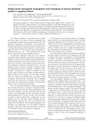
JOURNAL OF APPLIED PHYSICS 108, 024902 2010A low-cost millimeter wave interferometer for remote vibration sensingMartin L. Smith, 1 John A. Scales, 2,a Manoja Weiss, 3 and Brian Zadler 21 Blindgoat Geophysics, 2022 Quimby Mtn. Rd., Sharon, VT 05065, USA2 Department of Physics, Colorado School of Mines, Golden, Colorado 80401-1887, USA3 Division of Engineering, Colorado School of Mines, Golden, Colorado 80401-1887, USAReceived 9 January 2010; accepted 17 May 2010; published online 20 July 2010Remote sensing of ground vibration is a key tool in the detection of shallowly buried objects, suchas land mines. Millimeter wave systems show promise for replacing laser Doppler vibrometers asthe key sensing technology on the grounds of reduced cost and because they provide a larger 10 cmversus 1 mm, more robust sensor footprint. We have developed a double-conversion interferometeroperating at 39 GHz that can be built for about $10 000. The system employs quadrature detectionin order to provide reliable sensitivity over wavelength-sized changes in target range. Laboratorytests show that it can estimate sinusoidal ground motion from a 1 s time series with an uncertaintyof about 5 m. © 2010 American Institute of Physics. doi:10.1063/1.3452347I. INTRODUCTIONOne useful approach to the remote detection of shallowlyburied objects, such as antipersonnel mines, is basedupon how such objects modify the ground’s response to mechanicalvibration in the range of several hundred to severalthousand hertz. Some buried mines, for example, resonate inthis frequency range and their presence alters the ground’sresponse in ways visible in the spatial pattern of surfacemotion. 1 Excitation is typically provided by a remote acousticsource remote in this context may mean just a few centimetersto several meters and the ground response is mostcommonly mapped with a commercial laser vibrometer e.g.,Ref. 2.Laser vibrometers are expensive, extremely precise,fairly delicate, and have small sensing areas. We decided toreplace the laser vibrometer with a microwave device operatingin the millimeter wave band. Millimeter wavesMMWs span the frequency range from about 30 to 300GHz, with corresponding wavelengths of 1 cm–1 mm. Manycommercial applications have started to appear in this range,including automotive radar and point-to-point communication,and as a result millimeter wave components such aswaveguide, filters, harmonic multipliers/detectors, oscillators,etc., are becoming more widely available and at reasonablecost. In addition to lowered costs, wide availabilitybrings enhanced product variety and reduced lead times,which means that millimeter wave systems can be prototypedrelatively rapidly and changes in design can be quicklyevaluated.Applications of interest to us involve measuring displacementof the ground surface due to mechanical wavestraveling near the surface. These waves typically travel atspeeds of the order of 200 m/sec and have frequencies of10 2 –10 3 Hz. 2 Wavelengths are of the order 0.2–2.0 m.It is helpful to have a sensor which averages over lengthsup to about 0.1 M , where M is the wavelength of the mechanicalsignal of interest, in order to smooth out variabilitya Electronic mail: jscales@mines.eduin the soil. This amounts to a sensor footprint of 20–200 cm.The collimated beam of the system described here starts at awidth of 15 cm, which generally compares favorably withour requirements. By contrast a laser vibrometer has a spotsize of a few millimeters and can be expected to be muchmore affected by small-scale variability at the target site.II. SYSTEM CONFIGURATIONInitial tests with a low-cost 24 GHz Gunnplexer wereencouraging. 3 A Gunnplexer integrates a Gunn diode sourceand diode detector into a cavity coupled to a horn antenna; itis a simple, low-cost device and is popular in relatively undemandingapplications such as the radar guns used to enforcetraffic speed laws. We developed the system describedhere to ameliorate some of the Gunnplexer’s shortcomings asfollows:• The spectral purity of a free-running Gunn diode ispoor and contributes additional noise to the system.• There is no gain before the mixer which makes thesystem’s performance critically dependent on the noisefigure of the mixer.The system we built is a double-conversion superheterodyneconfiguration terminated in a quadrature detector. All ofthe components used are commercial, off-the-shelf items.The system operates at 39 GHz and has intermediate frequenciesIFs of 2.4 GHz and 10.0 MHz. Quadrature detectionat 10.0 MHz provides a baseband signal. All of theoscillators in the system are locked to a master oscillator.Our frequency-conversion scheme is built around a 6harmonic multiplier HM in the transmitter circuit and a 6 harmonic mixer HX in the receiver circuit. They aredriven, respectively, by local oscillators at 6.5 and 6.1 GHz.The actual rf of our interferometer is six times the frequencyof the local oscillator driving the HM6 6.5 GHz = 39 GHz.The received signal is passed through a 39 GHz low-noiseamplifier to the HX. Its injection frequency is0021-8979/2010/1082/024902/5/$30.00108, 024902-1© 2010 American Institute of Physics

024902-2 Smith et al. J. Appl. Phys. 108, 024902 20106 6.1 GHz = 36.6 GHz,leading to a first IF of 2.4 GHz. The 2.4 GHz signal is thenmixed with a 2.41 GHz signal resulting in a 10 MHz secondIF. This, in turn, goes to a quadrature demodulator driven atthe second IF 10 MHz, leading to baseband in-phase Iand quadrature Q outputs. The baseband outputs are routedto a pair of 1 kHz antialias filters and thence to a two-channeldigitizer providing 14 bits at a 10 kHz sample rate. Thetransmitted and reflected MMW signals are coupled from Kaband waveguide into a 15 cm Quinstar circular horn/lens viaa rectangular-circular transition. This produced a collimatedMMW beam.The master clock is a rubidium oscillator; surplus modelsare available for a few hundred dollars on eBay. Ours isa Stanford model. Since we only require short-term oscillatorstability, a high-quality quartz oscillator should work fineas an alternative. The rubidium units are internally just crystaloscillators with long-term stability controlled by a rubidiumvapor cavity. We use a distribution amplifier to amplifythe 10 MHz reference signal and provide 50 outputsfor all the oscillator synchronization inputs.The source of the 2.41 GHz injection for the secondmixer is a high-quality Anritsu synthesizer locked to themaster rubidium clock. In development it was very helpful tohave a sweepable oscillator so we could “go hunting” forsignals. There is no practical or theoretical obstacle to simplyreplacing this unit with a low-cost fixed oscillator, providedit can be phase-locked to the master 10 MHz clock. Bothlocal oscillators, as well as the 2.41 GHz synthesizer, werephase-locked to the 10 MHz that also served as the localoscillator for the final quadrature detector. Phase coherenceis essential to the instrument’s function as an interferometer.The system is broadband. We expect it to be flat in itsresponse to target movement for frequencies up to about 1MHz, or one-tenth of 10 MHz, the lowest rf signal in thesystem.The 6 HM and HX were made by TRW Milliwave. Thelocal oscillators at 6.5 and 6.1 GHz were purchased fromMicrowave Dynamics. The low-noise amplifier is from Quinstar.The 2.4 GHz detector and the 10 MHz quadrature detectorwere purchased from Minicircuits. All of these unitswere acquired at retail except for the HM and HX, whichwere purchased on eBay.A block diagram of the rf system is shown in Fig. 1.Based on our experience, the components shown in Fig. 1together with a satisfactory 10 MHz master clock could beassembled for about $10 000.Kim 4 describes a more sophisticated system which usesan additional IF to enhance selectivity and thus to reduceimage noise. He also develops a more sophisticated postprocessingsystem which, unlike ours see below, can tracktarget motions which are large compared to an rf wavelength.Finally he implements all of this in an integrated circuit. Wefound his descriptions and insights very helpful.x6~FIG. 1. Block diagram of the MMW interferometer described in the paper.All three oscillators are phase-locked to a master 10 MHz clock. The twobaseband outputs from the quad detector at the bottom of the diagram arethe in-phase and quadrature components.III. SIMPLE INTERFEROMETER THEORYConsider a target moving along the interferometer axis.Let r 0 be the average range to the target and t be theinstantaneous departure from the average range. The timedependentrange to the target isrt = r 0 + t.The signal received by the interferometer isSt = Atsin T t + t,where At accommodates amplitude changes due to rangechanges, T is the transmitter frequency, andt = 4 r 0 + t,is the two-way phase delay from interferometer to target.If At and t vary slowly at timescales of 0.1 sthe period of the last and smallest IF, then to a good approximationthe effect of each mixer stage in the receiverelectronics is to translate the frequency in Eq. 2 to a newreduced IF, change the amplitude by a constant factor, andadd a /2 phase shift. The in-phase component of thequadrature detector amounts to translating to 0. Ignoringamplitude changes, the result is the in-phase outputIt = 2A cost,1234= 2A cos 4 r 0 + t. 5Assume that t and expand Eq. 5 asIt = 2A cos 0 − 4 sin 0t,where 0 =4r 0 /. Filtering away the constant term leaves6

024902-3 Smith et al. J. Appl. Phys. 108, 024902 2010absolute peak-peak target velocity (mm/sec)1010.1measured0.09 + 4.29 * drive0.01 0.1 1drive signal (volts peak-peak)volts210Q (idle)I (idle)Q (driven)I (driven)FIG. 2. Crosses mark the velocity of the target as measured by a laservibrometer as a function of the drive signal at 40 Hz.It = 8At sin 0t. 7Let f˜ be the Fourier transform of ft. Assuming At=A 0 , a constant, thenĨ = 8A 0 sin 0˜,8tells us that the Fourier transform of t is directly proportionalto the Fourier transform of the observed quantity It.This result is compromised by the term sin 0 , which makesthe computation critically sensitive to the source-target separation.We can avoid this sensitivity by exploiting the second,quadrature, component of the quadrature detector.The quadrature channel is generated by mixing the incomingsignal with a copy of the local oscillator that hasbeen phase-shifted by /2. Working through the above derivationfor the phase-shifted signal leads toQ˜ = 8A 0 cos 0˜.9Quadrature detection is essential because either of the I s orQ s components may become small at a particular range becauseof the effect of the respective term cos 0 andsin 0 . We may combine the two components to computethe power spectrum of tP˜ = Ĩ 2 + Q˜ 2 .Substituting Eqs. 8 and 9 leads toP˜ = 8A 2 ˜ 2 ,1011which is independent of changes in the average range r 0 .Werefer to the spectrum obtained via Eq. 10 as the compositespectrum.IV. MEASURED PERFORMANCE0 0.05 0.1secondsFIG. 3. Color online Four time series showing the quadrature and in-phasesignals from the system when the shaker is idle top and driven at a peakvelocity of 4.4 mm/s at 40 Hz bottom.To test the performance of our system we attached atarget consisting of a small aluminum sheet to a B&K electromechanicalshaker driven by a signal generator. We calibratedthe plate vibration using a Polytec laser Doppler vibrometer.Figure 2 summarizes the laser Dopplermeasurements used to calibrate the shaker over applied voltagesfrom 20 mV PP to 1 V PP at 40 Hz. The latter, i.e.,1 V PP , we shall refer to as the driven state. The calibrationshows that the driven state corresponds to a total target speedof 4.4 mm/s or about4.4 mm=17 m,2 40in displacement at 40 Hz.We made measurements with our MMW system about 3m from the target, which was located inside of a home-mademicrowave anechoic chamber: a wooden box lined with Eccosorbmicrowave absorbing foam. Shown in Fig. 3 are fourtime series, for the in-phase and quadrature baseband outputs,in volts, for two conditions of target excitation. In theidle state no excitation voltage is applied to the shaker.V. SPECTRAL ANALYSIS THEORYIn order to characterize the performance of our instrumentwe wish to analyze the recorded signals to estimate1 The noise level in the recordings near the signal from amoving reflector and2 the level of the harmonic signal produced by a givenamount of physical motion of the reflector.We are also interested in any anomalous features in thespectrum that lie outside the range of random fluctuations.In this analysis we will use, and advocate, David Thomson’sscheme for multitaper Fourier transforms MTFTs.This approach has been extensively developed and appliedby Thomson and his colleagues, 5 but is still not in commonuse. Percival and Walden 6 offer a comprehensive, very readableexposition with numerous examples.An inherent property of digital Fourier transformsDFTs is that the computation actually yields the Fourieramplitudes for a time series of infinite length consisting ofrepeated copies of the observed time series, suitably normalizedto make the results bounded. Thus the Fourier transformwe actually compute is for the series which has repeateddiscontinuities at the points where the original, finite-lengthseries repeats. These jumps are unphysical: they are a consequenceof the DFT algorithm.

024902-4 Smith et al. J. Appl. Phys. 108, 024902 2010-40-60absorbertarget-40-50IQcomp-40-50dBdB-60-60-80-70-70-10010 20 30 40 50 60 70Hz-805 10 15Hz35 40 45Hz-80FIG. 4. Color online The upper curve shows the composite Fourier powerspectrum of the signal acquired when the interferometer was aimed at anoscillatory target in the driven state. The lower curve is the composite spectrumfor data acquired when the interferometer was aimed at an absorbingsurface.FIG. 5. Color online Power spectrum of the driven time series emphasizingthe regions 5–15 and 35–45 Hz which show strong spectral features. Thepeak at 40 Hz is the driven motion of the target, the other peaks are ofunknown origin. The figure shows the in-phase, quadrature, and compositecomponents of the spectrum.A conventional estimate of the power spectrum of a randomprocess is made by selecting and applying a taper beforecomputing the Fourier transform. A taper is a smoothfunction over the time domain which goes smoothly to zeroat the time series end-points and is typically, though not necessarily,non-negative. The role of a taper, as we think of it,is to ameliorate the high-frequency energy injected into thespectrum by the discontinuity between the first and lastpoints in the original time series. The taper also acts tosmooth the power spectrum over frequency and thus to reducethe variance in the estimated power at each frequency atthe cost of frequency resolution. When we choose a taperfrom a long menu of standard types we are choosing aspectral smoother. This means we are losing spectral definitionbut gaining robustness in the spectral power estimates,though we are often blissfully unaware of the character of thetradeoff. A common criticism of conventional tapers is thatthey discard some portion of the observed signal and thusunavoidably discard information.MTFT methods, in contrast, require an explicit choice ofan averaging window length and use that choice to constructan optimized taper which makes efficient use of nearly all ofthe data in the time series. The optimized taper is a linearcombination of members of a family of prolate spheroidalwave functions 7 associated with a given averaging length.These methods also provide a scheme, explicated in Ref. 6and which we use below, for estimating the amplitude ofspectral line components in the presence of noise. This approachprovides an accurate estimate of both the amplitudeof the line component as well as the residual spectrum leftafter removal of the line referred to as the reshaped spectrum.VI. DATA ANALYSISWe chose a spectral averaging window with a half-widthof four Fourier bins. For our 10 s data sets, this gives ahalf-width of 0.4 Hz. Figure 4 shows the composite Fourierpower spectra for data taken when the interferometer wasaimed at the target in the driven state upper curve and whenthe interferometer was aimed at an absorbing surface lowercurve. The spike at 40 Hz in the upper curve is the signalfrom the vibrating target. The origin of the other spikes isunknown but the large difference between the two curves,roughly 15–20 dB, suggests to us that all of the structure inthe upper curve arises one way or another from changes inthe apparent interferometric path length. They could represent,for example, additional motions of either the target orthe interferometer due to vibration induced by equipment orthe room environment.Figure 5 shows the details in the driven power spectrumin the region around the forced target motion right half andthe region 5–15 Hz which showed other, somewhat smaller,spectral lines. The width of the lines reflects the smoothinglength of the MTFT algorithm, but notice that the smoothingalgorithm preserves the sharp transitions between peak andbackground. The figure actually shows three trackingcurves. The highest is the composite signal while the othertwo are the in-phase and quadrature signals. Notice that theratio of the in-phase to the quadrature component, a quantitythat is sensitive to target range, is generally preserved acrossthe plot. This lends considerable weight to the view that allof these signals have been reflected from the target.We used multitaper spectral analysis 6 to estimate the lineamplitudes at 40 Hz in the two driven series and foundA I = 7.14 1.9 mV PK ,A Q = 5.81 1.6 mV PK .The composite demodulated amplitude is the vector sum ofthe I and Q sinusoidal amplitudes, per Eq. 10A = 9.2 2.4 mV PKFigure 6 shows the power spectral density of the driven compositedata series as well as that of the series after the estimatedsinusoidal term has been removed, the reshaped series.In our case the persistent signal has been reduced byabout 21 dB but there is still a substantial residual about 10dB above the local baseline. The residual signal must arisefrom effects that are not perfectly synchronous with the 40Hz motion of the target.

024902-5 Smith et al. J. Appl. Phys. 108, 024902 2010-40-50originalreshaped-20-30-40no tapermulti-taperdB-60dB-50-60-70-70-8030 35 40 45 50Hz-805 10 15HzFIG. 6. Color online Power spectrum of the driven time series, labeledraw, as well as of the time series after the estimated sinusoidal term has beenremoved, labeled reshaped.The estimated standard deviation of A is based on thenoise level remaining in the vicinity of A after the spectrumhas been reshaped. As we noted, that level is about 10 dBgreater than the local baseline. Since the variance of the lineestimate is proportional to the power spectral density, we cancorrect for this problem by reducing the standard deviationby the square root of the spectral amplitudes, or a factor ofabout 0.32A = 9.2 0.7 mV PK .Thus the standard deviation in the line amplitude due to ourestimate of the random noise in the system at 40 Hz is 0.7mV. Since a line amplitude of 9.2 mV corresponds to17 m, the standard deviation represents about 1.3 m ofdisplacement. Finally, these values are for a data series 10 slong. The variance due to noise is proportional to the inverseof the time series length at a fixed sampling rate. Ifweadjust the standard deviation to account for a 1 s serieslength, then we find a standard deviation of A of 4.1 m ofdisplacement.In order to highlight the differences between the untaperedand multitapered computations of power spectrum,Fig. 7 compares the two results for a portion of the powerspectrum of the inphase, driven data, and for the frequencyrange displayed in the left half of Fig. 5. It is clear that themultitaper spectrum has much less variance as well as poorerfrequency resolution. Linelike features acquire a half-widthof 0.4 Hz, but it is much more obvious which features in thespectrum are statistically significant. The loss of frequencyresolution is partly compensated by the ability of MTFTmethods to accurately detect, estimate, and remove line componentswith statistically well-founded methods, as discussedin Ref. 6.FIG. 7. Color online Power spectrum of the in-phase, driven data seriescomputed with no taper just a DFT compared to the results of the multitaperalgorithm. Note that the latter has both less variance as well as lessfrequency resolution.VII. CONCLUSIONSThe use of a millimeter wave microwave interferometeras the displacement sensor in standoff systems to detect shallowlyburied objects has a number of potential advantagesover traditional laser-Doppler vibrometers. Millimeter wavescan see through foliage and other optically opaque materials.Further, surface roughness is much less an issue than with alaser. For around $10 000 we were able to construct a highqualitymillimeter wave interferometer capable of measuringlow-frequency target motion with micron accuracy fromstand-off distances of a few meters. The entire system wasbuilt with off-the-shelf components and operates at just under40 GHz. We used modern multitaper spectral methods toestimate power spectral densities with rigorous uncertainties.ACKNOWLEDGMENTSThis work was partially supported by the Army ResearchOffice under Grant No. W911NF-07-1-0478.1 Dimitri M. Donskoy, in Alternatives for Landmine Detection, edited by J.MacDonald, Appendix H RAND, Santa Monica, CA, 2003.2 M. J. Sabatier and N. Xiang, Proc. SPIE 3710, 215 1999.3 T. Dylan Mikesell, K. van Wijk, J. A. Scales, and J. R. Peacock, Geophys.Res. Lett. 32, L01308 2005.4 S. Kim, Development of millimeter wave integrated-circuit interferometricsensors for industrial sensing applications, Ph.D. thesis, Texas A&M University,2004.5 D. J. Thomson, Bell Syst. Tech. J. I, 561977.6 B. D. Percival and A. T. Walden, Spectral Analysis for Physical ApplicationsCambridge University Press, Cambridge, UK, 1993.7 D. Slepian, Bell Syst. Tech. J. V, 571978.