ME6204 Convective Heat Transfer - National University of Singapore

NATIONAL UNIVERSITY of SINGAPORE
Department of Mechanical Engineering
ME6204 Convective Heat Transfer
Term Paper
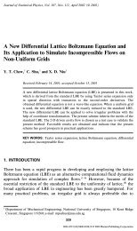
Laminar Flow and Heat Transfer from a Circular Cylinder in
Cross-flow using by the Lattice-Boltzman Method
Lecturer: Professor Arun S. Mujumdar
Submitted by
WU JIE
ZENG HUIMING
(g0500388@nus.edu.sg)
(g0500326@nus.edu.sg)

SINGAPORE
28 Feb 2006
1. Introduction
During the last two decades, as an alternative computational fluid dynamics
approach, the Lattice Boltzmann method (LBM) has achieved considerable success in
fluids engineering. Unlike traditional CFD methods, which are based on the
discretization of the macroscopic continuum equations, the LBM is based on the
microscopic models , mesoscopic kinetic equations, and the macroscopic dynamics of
a fluid is the result of collective behavior of many microscopic particles in the system.
The LBM has been proved to recover the Navier-Stokes equation by using the
Chapman-Enskog expansion. For more detail, reference [1] can be used.
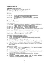
Figure1.1 Three levels of description of natural phenomena
The fundamental idea behind the LBM is the construction of simplified kinetic
models that incorporate the essential physics of microscopic or mesoscopic processes
so that the macroscopic averaged properties of the LBM obey the desired macroscopic
hydrodynamics. The basic premise of using these simplified kinetic-type method for
macroscopic fluid flows is that the macroscopic dynamics of a fluid is the results of
the collective behavior of many microscopic particles in the system and the
macroscopic dynamics is not sensitive to the underlying details in microscopic
physics.
The major advantages of the LBM are its explicit feature of the governing equation
- lattice Boltzmann equation, easy for parallel computation and easy for

implementation of complex boundary conditions.
On the other hand, in order to solve the problem about heat transfer, it is necessary
to consider the changing of temperature field in the domain. Since there is no very
successful thermal model in LBM, we use the macroscopic equation to implement the
variation of temperature in the fluid field.
2. Methodology
In our simulation, we use the lattice Boltzmann method to simulate the variation of
fluid density and velocity, while the changing of temperature field is governed by the
macroscopic energy equation.
The standard two-dimensional lattice Boltzmann equation can written as
1
fα α
t t t fα t fα t fα
t
τ
( )
eq
( x + e δ , + δ ) − ( x, ) = − ( x, ) − ( x , ) ( 0,1, 2, , M )
where f ( , t)
f
( , t)
α = L (2.1)
x is the density distribution function; α
eα
is the particle discrete velocity;
eq
α
x is its corresponding equilibrium distribution function, which depends on the
local macroscopic variables ρ andu ; τ is the single relaxation time; and M is the
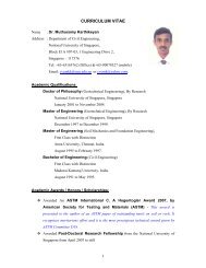
number of particle discrete velocity. Here, we choose the D2Q9 particle model, and
so M = 8 . The diagram is sketched in Fig 2.1.
Fig 2.1 D2Q9 model
For the D2Q9 model, the particle discrete velocity is defined as:

( )
⎪
⎨( ⎡⎣ ( ) ⎤⎦ ⎡⎣ ( ) ⎤⎦
)
⎪
( ⎡ ( ) ⎤ ⎡ ( ) ⎤)
e = cos π α −1 4 ,sin π α − 1 4 , α = 1,3,5,7
(2.2)
α
⎧
0,0 , α = 0
⎪ 2 cos ⎣π α −1 4 ⎦ ,sin ⎣π α − 1 4 ⎦ , α = 2,4,6,8
⎩
and the equilibrium distribution function is:
9 2 3
= ω ρ ⎡
⎢
1+ 3( ⋅ ) + ( ⋅ ) − ( ⋅ )
⎤
⎣
e u 2 e u 2
u u ⎥
⎦
(2.3)
eq
f α α α α
where the coefficientωα
is:
⎧4 9, α = 0
⎪
ωα
= ⎨1 9, α = 1,3,5,7
⎪
⎩1 36, α = 2, 4,6,8
(2.4)
The macroscopic density ρ and momentum density ρu can be computed as:
8
f α
α = 0
ρ = ∑ ;
8
f α α
α = 1
ρu = ∑ e (2.5)
The equation of state and kinematic viscosity can be defined as:
P c s
2
= ρ
(2.6)
2
s
( 0.5)
υ = c τ − δ t
(2.7)
where
2
cs
is speed of sound, for D2Q9 model, it is equal to1 3.
Since the standard lattice Boltzmann equation uses the uniform mesh, in order to
extend this method to the non-uniform grid, the modification is necessary. Here, we
choose the Taylor series expansion- and Least square based-lattice Boltzmann method.
The two-dimensional governing equation is
( δ )
α 0 0 α1 α1, α −1
j=
1
9
f x , y , t + t = V = ∑ a
j
g
j
(2.8)
where
a α 1, j
is a set of coefficients, which can be computed in advance;
j 1
g α −
is
1
g
1 ( 1, ) ( ( 1, ) eq
α j− = fα j − t − fα j − t − fα
( j − 1, t)
) 1,2, ,9
τ
j = L (2.9)
Obviously, it is a simple algebraic equation and is easy to solve. Details are in
reference [2].

The macroscopic energy equation governing temperature changing [6] is
2 2
( uT ) ( vT ) λ
∂T ∂ ∂ ⎛ ∂ T ∂ T ⎞
+ + = ⎜ +
2 2 ⎟
∂t ∂x ∂y ρcp
⎝ ∂x ∂y
⎠
(2.10)
where T is temperature; u,
v are the velocities of fluid; λ is the thermal
conductivity; ρ is density;
cp
is fluid specific heat capacity. The term λ ρcp
can
UD
be written as , where U is characteristic velocity; D is characteristic length,
Re Pr
here refers to the diameter of cylinder; Re is Reynolds number and Pr is Prandtl
number.
In order to solve the above equation in the non-uniform grid, we use the coordinate
transfer to transfer equation from ( x,
y ) to ( , )
∂ T uyη − vxη vxξ − uxξ
UD
+ + = − +
∂t J J
ξ η . The final equation is
2
Tξ Tη {( αTξξ 2βTξη γTηη
) J
Re Pr
3
( α xξξ 2β xξη γ xηη )( yξTη yηTξ ) ( α yξξ 2β yξη γ yηη )( xηT ξ
xξTη
) ⎤ J }
+ ⎡
⎣
− + − + − + −
⎦
where
α = x + y ; β = x x + y y ;
2 2
η η
ξ η ξ η
γ = x + y ; J = x y − x y .
2 2
ξ ξ
ξ η η ξ
The derivatives in the above equation can be discretized using center difference
except for the term of convection. The term of convection can be discretized by
windward scheme of third order
( + + − − )
( + + − − )
⎛ ∂T
⎞
⎧
⎪ fi, j
Ti 2, j
− 2Ti 1, j
+ 9Ti , j
− 10Ti 1, j
+ 2Ti 2, j
6∆ξ
fi,
j
≥ 0
⎜ f ⎟ = ⎨
⎝ ∂ξ
⎠i, j ⎪ ⎩
fi, j
− 2Ti 2, j
+ 10Ti 1, j
− 9Ti , j
+ 2Ti 1, j
−Ti 2, j
6∆ ξ fi,
j
< 0
where
f
uyη
− vxη
= . And
J
( + + − − )
( + + − − )
⎛ ∂T
⎞
⎧
⎪ fi, j
Ti 2, j
− 2Ti 1, j
+ 9Ti , j
− 10Ti 1, j
+ 2Ti 2, j
6∆η
fi,
j
≥ 0
⎜ f ⎟ = ⎨
⎝ ∂η
⎠i, j ⎪ ⎩
fi, j
− 2Ti 2, j
+ 10Ti 1, j
− 9Ti , j
+ 2Ti 1, j
−Ti 2, j
6∆ η fi,
j
< 0
where
f
vxξ
− uxξ
= . See reference [8].
J
3. Results and Discussion
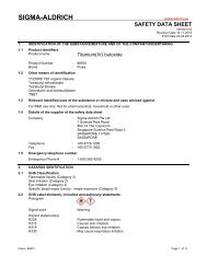
In our simulation, we use O-type body fit mesh, as shown in Fig 3.1.

Fig 3.1 O-type body fit grid
Here, the Reynolds number is defined as Re
UD
= , the Prandtl number is
υ
µc
Pr =
p
. We set the kinematic viscosity, υ = 0.01, free stream velocity
λ
and Prandtl number Pr = 0.7 ( fluid is air ).
Boundary conditions:
U
Re⋅υ
= ,
D
Initially, the temperature of fluid is T
0
= 298.15 K, the temperature of cylinder is
KTw = 473.15, the fluid is stationary except that the far field has the free stream
velocity.
The density distribution function f α
in the whole domain is equal to its
corresponding equilibrium distribution function,
eq
f α
.
During the process of computation, the temperature of far field and cylinder
invariable; at the same time, the velocity of far field constant, equaling to free
stream velocity; and the velocity of the surface of cylinder is zero (no-slip
condition).
The distribution function f α
satisfies the bounceback rule at the surface of
cylinder; while at the far field, the distribution function f α
is set to be equal to

the equilibrium distribution function
eq
f α
.
3.1 Temperature and pressure patterns
In our simulation, six different Reynolds numbers are selected: 4, 20, 40, 100, 160
and 1000. First, the temperature and pressure patterns are given.
Reynolds number: 4
Reynolds number: 20
Reynolds number: 40

When the Reynolds number 1≤Re≤40, the flow is steady, and both upstream and
downstream is symmetrical. Therefore, the temperature and pressure patterns are
symmetrical as well. At the same time, when the Reynolds number is low (Re=4), the
thickness of the thermal layer is high. With the increment of Reynolds number, we
find that the thickness of thermal layer becomes lower.
Reynolds number: 100
Reynolds number: 160
When the Reynolds number 50≤Re≤160, the flow becomes unsteady and periodic.
The Karman vortex streets appear and dominate the flow domain finally.

Reynolds number: 1000
When the Reynolds number Re=1000, the flow is turbulent.
3.2 Streamlines and vorticity contours
At the same time, we also give the streamlines and vorticity contours at different
Reynolds numbers.
Streamline (left) and vorticity contours (right) (Re=4)
Streamline (left) and vorticity contours (right) (Re=20)

Streamline (left) and vorticity contours (right) (Re=40)
From the above the diagrams, we can find that, when the Reynolds number is low
the streamline can keep close to the surface of cylinder. Enhancing the Reynolds
number, a couple of vortex would appear behind the cylinder. The size of vortex
could increase with the Reynolds number.
Streamline (left) and vorticity contours (right) (Re=100)
Streamline (left) and vorticity contour (right)
(Re=160)

The above figures indicate that the size of Karman vortex street also increases with
Reynolds number.
3.3 Velocity patterns
Streamline (left) and vorticity contours (right) (Re=1000)
Re=4
Re=20
Re=40
Re=100

Re=160
Re=1000
3.4 Pressure coefficient along the cylinder
p − p0
The pressure coefficient along the cylinder is defined asCp
= .
1 2
ρ0U
2
Re=4
Re=20
Re=40
Re=100

Re=160
Re=1000
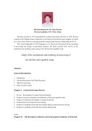
3.5 Nusselt number along the cylinder
∂T
The Nusselt number is defined as Nu = − . ∂ n
Re=4
Re=20
Re=40
Re=100

Re=160
Re=1000
Here, we define the zero angle at rear point of cylinder, and angle increases along
the anti-clockwise direction. The above diagrams show variation of the average
cylinder Nusselt number. The front surface consistently displays the highest Nusselt
number, the top and bottom surface value is intermediate, followed by the rear surface.
The rear Nusselt number is more strongly dependent on the Reynolds number in the
unsteady periodic flow as compared to the steady flow regime.
4. Conclusions
This study focuses on the unconfined flow and heat transfer characteristic a round
cylinder in the two dimensions. The flow for Re≤40 is noted to be steady, while that
for Re≥50 is periodic, with the transition to unsteadiness occurring between Re=40
and Re=50. This agrees with prior experimental and computational studies.
The primary focus of this study, however, has been the heat transfer from the
cylinder by LBM, which has not been extensively studied previously. The cylinder
average Nusselt number increases with increasing Reynolds number. Finally, heat
transfer correlations applicable in 2-D flow regime have been proposed for both the
temperature boundary conditions considered.
The Lattice Boltzmann method is an efficient approach for the computational fluid
dynamics. The major advantage of this method is that its governing equation is very
simple, and it is also easy to implement by programming. In order to solve the
problem of heat transfer, only the macroscopic energy equation is included. From the

above illustration we find that, using LBM along with the energy equation gives
satisfactory results.
Reference
1. S. Chen and G. D. Doolen, “Lattice Boltzmann Method for Fluid Flows”, Annu. Rev. Fluid
Mech, 1998(30), pp329-364.
2. C. Shu, X. D. Niu and Y. T. Chew, “Taylor-series Expansion and Least Squares-based Lattice
Boltzmann Method: Two-Dimensional Formulation and Its Applications”, Physical Review E,
2002(65), 036708.
3. Ganesan P., Loganathan P., “Unsteady natural convective flow past a moving vertical cylinder
with heat and mass transfer”, Heat Mass Tranfer, 2001(37), pp.59-65.
4. Eagles P.M., Soundalgekar V. M., “Stability of flow between two rotating cylinders in the
presence of a constant heat flux at the outer cylinder and radial temperature gradient - wide gap
problem”, Heat Mass Transfer, 1997(33), pp.257-260.
5. Armouzi M. El., Chesneau X., Zeghmati B., “Numerical study of evaporation by mixed
convection of a binary liquid film flowing down the wall of two coaxial cylinders”, Heat Mass
Transfer, 2005( 41), pp.375–386.
6. Eswaran V., Sharma A, “Heat and fluid flow across a square cylinder in the two-dimensional
laminar flow regime”, Numerical Heat Transfer, 2004(45), pp.247-269.
7. Lange C.F., Durst F., M. Breuer, “Momentum and Heat Transfer from Cylinders in Laminar
Crossflow at
4
10 −