Stokes Equation - Solution in Spherical Polar Coordinates
Stokes Equation - Solution in Spherical Polar Coordinates
Stokes Equation - Solution in Spherical Polar Coordinates

Create successful ePaper yourself
Turn your PDF publications into a flip-book with our unique Google optimized e-Paper software.
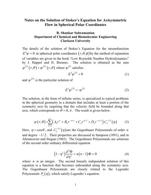
Notes on the <strong>Solution</strong> of <strong>Stokes</strong>’s <strong>Equation</strong> for Axisymmetric<br />
Flow <strong>in</strong> <strong>Spherical</strong> <strong>Polar</strong> Coord<strong>in</strong>ates<br />
R. Shankar Subramanian<br />
Department of Chemical and Biomolecular Eng<strong>in</strong>eer<strong>in</strong>g<br />
Clarkson University<br />
The details of the solution of <strong>Stokes</strong>’s <strong>Equation</strong> for the streamfunction<br />
4<br />
E ψ = 0 <strong>in</strong> spherical polar coord<strong>in</strong>ates ( r, θφ , ) by the method of separation<br />
of variables are given <strong>in</strong> the book “Low Reynolds Number Hydrodynamics”<br />
by J. Happel and H. Brenner. The solution is obta<strong>in</strong>ed as the sum<br />
1<br />
, 2<br />
( 1)<br />
ψ r θ + ψ r,<br />
θ where ψ satisfies<br />
( ) ( )<br />
( 2)<br />
( ) ( )<br />
and ψ is the particular solution of<br />
( 1)<br />
2<br />
E ψ = 0<br />
(1)<br />
2<br />
E ψ<br />
( 2) ( 1)<br />
= ψ<br />
(2)<br />
The solution, <strong>in</strong> the form of <strong>in</strong>f<strong>in</strong>ite series, is specialized to typical problems<br />
<strong>in</strong> the spherical geometry <strong>in</strong> a doma<strong>in</strong> that <strong>in</strong>cludes at least a portion of the<br />
symmetry axis by requir<strong>in</strong>g that the velocity field be bounded along that<br />
axis, which corresponds to θ = 0, π . The result is given below.<br />
∞<br />
∑ n n n n<br />
C<br />
n<br />
(3)<br />
n=<br />
2<br />
−1/2<br />
C<br />
n<br />
η are the Gegenbauer Polynomials of order n<br />
n − n+ 1 n+ 2 − n+ 3 −1/2<br />
( r,<br />
) = ( Ar + Br + Cr + Dr ) ( )<br />
ψ θ η<br />
Here, η cosθ<br />
and degree − 1/2. Their properties are discussed <strong>in</strong> Sampson (1891), and <strong>in</strong><br />
Abramowitz and Stegun (1965). The Gegenbauer Polynomials are solutions<br />
of the second order ord<strong>in</strong>ary differential equation<br />
= , and ( )<br />
2<br />
2 d Φ<br />
( 1− η ) + n<br />
2<br />
( n−1)<br />
Φ= 0<br />
(4)<br />
dη<br />
where n is an <strong>in</strong>teger. The second l<strong>in</strong>early <strong>in</strong>dependent solution of this<br />
equation is a function that becomes unbounded along the symmetry axis.<br />
The Gegenbauer Polynomials are closely related to the Legendre<br />
Polynomials ( ) n<br />
P η , which satisfy Legendre’s equation.<br />
1
d ⎡ 2 dΦ<br />
⎤<br />
( 1 η ) n( n 1)<br />
0<br />
dη<br />
⎢ − + + Φ=<br />
dη<br />
⎥<br />
(5)<br />
⎣ ⎦<br />
Many important properties of the Legendre Polynomials can be found <strong>in</strong><br />
MacRobert (1967) and <strong>in</strong> Abramowitz and Stegun (1965).<br />
Some useful relationships <strong>in</strong>volv<strong>in</strong>g the Gegenbauer Polynomials are given<br />
below.<br />
( η) − P ( η)<br />
P<br />
2n<br />
−1<br />
η<br />
−1/2<br />
C<br />
n ( η ) = − ∫ P<br />
1 ( )<br />
1<br />
n−<br />
s ds<br />
(7)<br />
−<br />
−1/2<br />
n−2<br />
n<br />
C<br />
n ( η ) =<br />
(6)<br />
The first few Gegenbauer and Legendre Polynomials are<br />
C<br />
C<br />
C<br />
P<br />
P<br />
P<br />
−<br />
( ) 1 C ( )<br />
η = η = η<br />
−1/2 1/2<br />
0 1<br />
1 1<br />
2 2<br />
1 1<br />
8 5 1<br />
−<br />
( η) = ( 1− η ) C ( η) = η ( 1−η<br />
)<br />
−1/2 2 1/2 2<br />
2 3<br />
( η) = ( −η )( η − )<br />
−1/2 2 2<br />
4<br />
( ) 1<br />
P ( )<br />
0 1<br />
2 2<br />
( η) = ( 3η − 1) P ( η) = η( 5η<br />
−3)<br />
2 3<br />
4<br />
η = η = η<br />
1 1<br />
2 2<br />
1 35<br />
8 30 3<br />
4 2<br />
( η) = ( η − η + )<br />
The Gegenbauer Polynomials satisfy the orthogonality property<br />
for values of mn≥ , 2.<br />
−1/2 −1/2<br />
+ 1<br />
m ( η) n ( η)<br />
2<br />
∫ C C dη<br />
=<br />
δ<br />
1<br />
2<br />
mn<br />
(8)<br />
−<br />
1−η<br />
n( n−1)( 2n−1)<br />
2
The function Qn<br />
( )<br />
−1/2<br />
Gegenbauer Polynomials through Q ( η) = −C ( η)<br />
.<br />
η used by Leal <strong>in</strong> the textbook is related to the<br />
n<br />
n+<br />
1<br />
References<br />
M.A. Abramowitz and I.A. Stegun, “Handbook of Mathematical Functions,”<br />
Dover Publications (1965).<br />
J. Happel, and H. Brenner, “Low Reynolds Number Hydrodynamics,”<br />
Prentice-Hall (1965); republished by Noordhoff International (1973).<br />
L.G. Leal, “Lam<strong>in</strong>ar Flow and Convective Transport Processes,”<br />
Butterworth-He<strong>in</strong>emann (1992).<br />
T.M. MacRobert, “<strong>Spherical</strong> Harmonics,” Pergamon Press (1967).<br />
R.A. Sampson, “On <strong>Stokes</strong>’s Current Function,” Phil. Trans. Royal Soc. A<br />
182, 449-518 (1891).<br />
3