Indirect gradient analysis - Alaska Geobotany Center

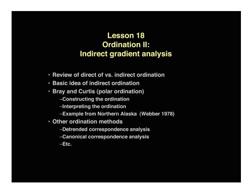
Lesson 18
Ordination II:
Indirect gradient analysis
• Review of direct of vs. indirect ordination
• Basic idea of indirect ordination
• Bray and Curtis (polar ordination)
–Constructing the ordination
–Interpreting the ordination
–Example from Northern Alaska (Webber 1978)
• Other ordination methods
–Detrended correspondence analysis
–Canonical correspondence analysis
–Etc.

Direct vs. Indirect ordination
Direct ordination examines vegetation changes along known environmental gradients (e.g. a
moisture gradient or elevation gradient).
Indirect ordination examines the environmental causes of vegetation patterns by first arranging
the stands or species according to their floristic similarity. Relationship of the stands to
environmental gradients is then achieved by either correlating the axes with environmental
variables or by determining the relationship of all the measured environmental variables with
the ordination space..

Vegetation
Ecosystem
Environmental
factors
Three main approaches to
analysis of vegetation data
Field description
(Sampling and measuring, Field phase of B-B
method)
Site factors
and soils
data
Rows: Species
names
Columns: Relevé/ plot
nos.
Relevé
species
data
Floristic Data
Matrix
(Data from relevé
species data form)
Rows:
Environmental
variables
Columns: Relevé/ plot nos.
Environmental
Data Matrix
(Data from relevé
site factor form, and
soils analysis)
1 3 2
Classification
Sorted Table
Analysis
(Analytical Phase of B-B
method)
Indirect
gradient
analysis
(Vegetation
ordination)
Ordination axes and
graphs derived from
species data.
Direct gradient
analysis
(Environmental
ordination)
Ordination axes and
graphs derived from
environmental data.
Cover or importance
of species plotted on
environmental axes.
1. Classification: Based solely on
floristic data matrix.
2. Direct gradient analysis: Axes
of ordination derived from
environmental data. Species
cover or importance plotted
along the axes.
3. Indirect gradient analysis:
Ordination derived solely from
species data. Environmental
data are then used to interpret
the ordination.
Patterns of plots or
species are shown
based on similarity.
Environmental data
introduced after
analysis to aid
interpretation.

Vegetation
Ecosystem
Environmental
factors
Field description
(Sampling and measuring, Field phase of B-B method)
Indirect Gradient Analysis
Approach
Species data are used to construct
the axes of the ordination
diagrams.
Site factors
and soils
data
Rows: Species
names
Columns: Relevé/ plot nos.
Floristic Data Matrix
(Data from relevé species
data form)
Rows: Environmental
variables
Columns: Relevé/ plot nos.
Environmental Data
Matrix
(Data from relevé site factor
form, and soils analysis)
1. Plots (relevés) are located
along the axes based on their
floristic similarity to each
other. (Or species can be
located based on the
similarity of their occurrence
within the plots.)
Relevé
species
data
Indirect gradient
analysis (Vegetation
ordination)
Ordination axes and graphs
derived from species data.
2
2. Environmental data are then
used to help interpret the
ordination.
• Coordinates of axes can be
correlated with the environmental
data.
• Trends of environmental
gradients can be plotted within
the ordination space (biplot
diagrams).
1
Patterns of plots or species
are shown based on
similarity. Environmental
data introduced after
analysis to aid interpretation.

Indirect gradient analysis
• “Indirect gradient analysis is a multidimensional picture of the relationships between stands
of vegetation based on their floristic similarity to each other (in the case of a plot ordination),
or between species based on their concurrence in vegetation plots (in the case of a species
ordination).”
• The first step is to calculate the similarity of each stand to all the others. This can be
done using a variety of similarity indices. This information is then arranged into a
similarity/dissimilarity matrix. The information is then used to construct an ordination
diagram, where every plot has an x and y coordinate.
• The x,y coordinates of stands or species in the multidimensional space are then
correlated with environmental information for each plot to detect possible
environmental gradients within the data set.

Goals of ordination
1. Show floristic relationships between stands of vegetation or between species.
The distances between points on the ordination are measures of their floristic
degree of similarity.
2. Reduce noise (unexplained variation that masks the similarity relationships
between species and/or plots)
3. Discover the underlying structure of the vegetation data that is due to
redundancy. The redundant nature of vegetation data is caused by sampling
similar stands of vegetation and is due to the coordinated species responses in
similar environments. Many vegetation samples have similar species
composition, presumably due to their occurrence in similar environments.

Plot ordinations vs. species ordinations
• In plot ordinations, each point represents a plot (relevé) and the greater the distance
between any two points, the greater the difference in floristic composition of the plots.
• In species ordinations, each point corresponds to a species point of central tendency.
Distances between species are an approximation of their degree of similarity in terms
of their distribution within plots.

Plot ordination
• Numbered points are
plots.
• Plots 19 and 15 are
very similar to each
other in terms of
species composition.
• Plots 19 and 25 are
dissimilar to each
other.
Detrended correspondence analysis of Gutter Tor data, Kent and Coker, 1992
• The axes are
functions of species
similarity and have no
environmental
meaning on their own,
but can be correlated
with environmental
data from the study
plots.
• The area contained by
the axes is called the
“ordination space”.

1-, 2-, and 3-dimensional plot ordinations
• These are are ordinations in 1, 2 and 3
dimensions, showing the arrangement
of plots according to their similarity to
each other.
• A 3-D ordination can reveal plots that
appear very similar to each other in 1-D
or 2-D space but that are actually quite
dissimilar (e.g., plots 7 and 10).

Plot and species ordinations
In plot
ordinations, the
columns are
the plot
(quadrat)
numbers and
the rows the
species names.
In species
ordinations, the
species matrix
is inverted and
the species are
the columns
and the rows
the plot
numberss.

Species ordination
Species ordinations
are interpreted
similar to plot
ordinations.
• Fig. 5.11, Kent and Coker
Species that are
close to each other
are likely to cooccur
in the
landscape (e.g.,
Trichophorum
caespitosum and
Juncus effusus.
Species that are far
apart probably do
not occur in the
same plots.
Kent and Coker, 1992

Interpreting the ordination diagram
• The axes of the ordination are gradients of floristic similarity (in the case of quadrat
ordinations) or gradients of plot-occurrence similarity (in the case of species
ordinations).
• The results of ordination can be displayed one, two or three dimensions which define
the ordination space.
• In general, the axes produced by ordination analysis come out in descending order of
importance. The first axis is most important and describes the most variation in the
floristic data.
• A powerful attribute of plot ordinations is that the plot numbers can be replaced with
species cover values or environmental data to portray trends of environmental
variables or species cover within the ordination space.

Relating the plot ordination to environmental data
One way to show
environmental relationships
is to construct separate
plots for each
environmental variable
sampled and then replace
the plot numbers in the
ordination with the value
from the appropriate
environmental variable.
Here the plot numbers have
been replaced with values
of pH, % soil moisture and
grazing intensity
respectively.

Relating the plot ordination to environmental data
pH4.5
If clear patterns exist,
isolines can be drawn to
show trends of
environmental variables
within the ordination
space.
GI>6
SM>90%
SM=41-60%
SM

Polar ordination
• Developed by Bray and Curtis (1957) to analyze the upland forests of
Wisconsin.
• Followed a fix set of rules that could be done by hand or by a computer.
• Based on Euclidian geometry.
• Easily understood and good method for teaching the fundamentals of
ordination.

1. Begin with the primary data matrix (rows=species, columns=plot numbers).
2. Calculate the similarity and dissimilarity matrices.
3. Compute the first axis and position all plots along it.
– The first reference stand is selected that has the least similarity to all other plots.
– The second reference stand is the one with the least similariy to the first. The
maximum possible dissimilarity between these plots is 100%. The dissimilarity
between the two stands defines the length of the first axis.
– Locate all the other plots with respect to these two reference stands based on
their geometric relationships:

Steps in calculation of the ordination
Wisconsin example data set
Plots
Species 1 2 3 4 5 6 7 8 9 10
Quercus
9 8 3 5 6 5
macrocarpa
Quercus velutina 8 9 8 7
Carya ovata 6 6 2 7 1
Prunus serotina 3 5 6 6 6 4 5 4 1
Quercus alba 5 4 9 9 7 7 4 6 2
Juglans nigra 2 3 5 6 7 3
Quercus rubra 3 4 6 9 8 7 9 4 3
Juglans cinerea 5 2 2 2
Ulmus americana 2 2 4 5 6 5 2 5
Tilia americana 2 7 6 6 7 6
Ulmus rubra 4 2 2 5 7 8 8 8 7
Carya cordiformis 5 6 4 3
Ostrya virginiana 7 4 6 5
Acer saccharum 5 4 8 8 9
Step 1.
Begin with the primary data
matrix (rows=species,
columns=plot numbers).
Values here are log cover
scores, 1-9.

Step 2. Calculate similarity and dissimilarity of all pairs of plots and make
similarity/dissimilarity matrix
The calculation of similarity is fairly
intuitive for the situation where two
plots have only
two species.
In this case, the Euclidian distance can
be calculated according to the
Pathagorean theorem.

Jaccard s and Sorenson s similarity indices
For situations with many plots and many species, a variety of similarity indices have
been developed. Jaccard s and Sorenson s indices are based on presence/absence of
species that are shared between samples of vegetation and species that are unique to each
sample.
Jaccard s similarity index:
IS J
=
a
a + b + c
a = number of species in common between the stands
b = number of species unique to the first stand,
c = number of species unique to the second stand.
Sorenson s similarity index:
IS S
= 2a
2a + b + c
Places more emphasis on the similarities.

Czenkanowski s index of similarity
Czekanowski s coefficient (IS c ) is a modification of Sorenson s similarity index that
considers the abundance (cover) of species:
ISc =
m
2 min( xi, yi)
i=1
m
i =1
x
i +
m
yi
i =1
Where the numerator is the sum of minimum cover value for each species (i)
in each pair of plots (x, y).
The denominator is the sum of the cover values for all species in stand x plus
the sum of the cover values for all species in stand y.

Similarity and dissimilarity for plots 2 and 9
Plots
Species 1 2 3 4 5 6 7 8 9 10
Quercus
9 8 3 5 6 5
macrocarpa
Quercus velutina 8 9 8 7
Carya ovata 6 6 2 7 1
Prunus serotina 3 5 6 6 6 4 5 4 1
Quercus alba 5 4 9 9 7 7 4 6 2
Juglans nigra 2 3 5 6 7 3
Quercus rubra 3 4 6 9 8 7 9 4 3
Juglans cinerea 5 2 2 2
Ulmus americana 2 2 4 5 6 5 2 5
Tilia americana 2 7 6 6 7 6
Ulmus rubra 4 2 2 5 7 8 8 8 7
Carya cordiformis 5 6 4 3
Ostrya virginiana 7 4 6 5
Acer saccharum 5 4 8 8 9
Total 38
42
ISc =
2 min( xi, yi)
i=1
m
IS 2,9 = 2(0+0+0+4+0+0+4+0+2+0+0+0+0+0)
38+42
Similarity = 20/80 = .25
m
i =1
x
i +
m
yi
i =1
Dissimilarity = 1-Is c
= 1-.25 = .75

Similarity for species Quercus macrocarpa and Q. velutina
Plots
Species 1 2 3 4 5 6 7 8 9 10
Quercus
9 8 3 5 6 5
macrocarpa
Quercus velutina 8 9 8 7
Carya ovata 6 6 2 7 1
Prunus serotina 3 5 6 6 6 4 5 4 1
Quercus alba 5 4 9 9 7 7 4 6 2
Juglans nigra 2 3 5 6 7 3
Quercus rubra 3 4 6 9 8 7 9 4 3
Juglans cinerea 5 2 2 2
Ulmus americana 2 2 4 5 6 5 2 5
Tilia americana 2 7 6 6 7 6
Ulmus rubra 4 2 2 5 7 8 8 8 7
Carya cordiformis 5 6 4 3
Ostrya virginiana 7 4 6 5
Acer saccharum 5 4 8 8 9
Total
37
32
ISc =
m
2 min( xi, yi)
i=1
m
i =1
x
i +
m
yi
i =1
IS Qm,Qv = 2(8+8+3+5+0+0+0+0+0+0)
37+32
Similarity = 48/69 = .696
Dissimilarity = 1-.696 = .304

Step 2. Matrices of similarities and dissimilarities
(Wisconsin Upland forest, Czenkanowski s index)
Matrix of similarities
Sample number 1 2 3 4 5 6 7 8 9 10
1 85 62 74 57 40 44 29 33 28
2 85 62 78 50 30 40 17 25 20
3 62 62 38 28 32 35 22 20 27
4 74 78 38 67 42 49 28 27 29
5 57 50 28 67 61 66 54 45 45
6 40 30 32 42 61 75 80 66 59
7 44 40 35 49 66 75 74 71 68
8 29 17 22 28 54 80 74 69 72
9 33 25 20 27 45 66 71 69 75
10 28 20 27 29 45 59 68 72 75
• Similarity indices based on
Czekanowski s similarity
index.
• Dissimilarity is 1 - S c
.
Matrix of dissimilarities
Sample number 1 2 3 4 5 6 7 8 9 10
1 15 38 26 43 60 56 71 67 72
2 15 38 22 50 70 60 83 75 80
3 38 38 62 72 68 65 78 80 73
4 26 22 62 33 58 51 72 73 71
5 43 50 72 33 39 34 46 55 55
6 60 70 68 58 39 25 20 34 41
7 56 60 65 51 34 25 27 30 32
8 71 82 79 72 46 20 27 31 28
9 67 75 80 73 55 34 30 31 25
10 72 80 73 71 55 41 32 28 25

Step 3. Compute first axis of the ordination and position all
plots along it
1. Sum all the similarities for each plot.
2. Select the plots at the ends of the first
axis. These are the plots that are least
similar to all the other plots and least
similar to each other. The plot at the left
end of the first axis has the lowest sum of
similarities, i.e. is least similar to all other
plots. Here Plot 3 is least similar to all the
others.
3. The plot at the right end of the first axis is
the one with the least similarity to the first.
Here Plot 9 is most dissimilar to Plot 3.
The maximum possible dissimilarity
between these plots is 100%. The
dissimilarity between the two stands
defines the length of the first axis.
4. Locate all the other plots with respect to
these two reference stands based on their
geometric relationships.

Calculation of x values along the 1st axis
A and B are the plots at the
ends of the first axis.
P is the plot to position with
reference to the A and B.
P has dissimilarity of dA with
reference to Plot A and
dissimilarity dB with respect
to Plot B.
Solving for x:
x 2 + e 2 = (dA) 2 , e 2 = (dA) 2 - x 2
(L-x) 2 + e 2 = (dB) 2
(L-x) 2 + (dA) 2 - x 2 = (dB) 2
L 2 - 2Lx + x 2 + (dA) 2 - x 2 = (dB) 2
L 2 - 2Lx + (dA) 2 = (dB) 2
x =( L 2 + (dA) 2 - (dB) 2 )/2L
Using a compass, P can be
positioned with respect to A
and B.
The perpendicular from P to
the first axis is e.
x is the distance of P from A
and is calculated by the
Pythagorean theorem.

Geometric determination of plots along the first axis
All the plots are positioned with
respect to reference plots 3
and 9.
For Plot 1, the dissimilarity to
Plot 3, d 1,3
, is 38, and
dissimilarity to Plot 9, d 1,9
, is
67. (See dissimilarity matrix.)
d 1,3 = 38
x 1,3 = 21
d 1,9 = 67
The x coordinate of plot 1 is:
x = (L 2 + (dA) 2 - (dB) 2 )/2L
X 1,3
= (80 2 + 38 2 - 67 2 )/(2(80)) =
(6400 + 1444 + 4489)/160 = 21

Geometric determination of plots along the first axis
Dissimilarity matrix:
All the plots are positioned with
respect to reference plots 3
and 9.
For Plot 1, the dissimilarity to
Plot 3, d 1,3
, is 38, and
dissimilarity to Plot 9, d 1,9
, is
67. (See dissimilarity matrix.)
d 1,3 = 38
x 1,3 = 21
d 1,9 = 67
The x coordinate of plot 1 is:
x = (L 2 + (dA) 2 - (dB) 2 )/2L
X 1,3
= (80 2 + 38 2 - 67 2 )/(2(80)) =
(6400 + 1444 + 4489)/160 = 21

Distances on the x axis
x = (L 2 + (dA) 2 - (dB) 2 )/2L
Distances on the first axis:
Calculate the distance along the x-axis of all stands in reference to stand 3 (first reference stand):
Use the geometric solution (K&C, p. 185) to calculate distance from stand 3:
Stand dA (dissim to 3) dB (dissim to 9) x
1 38.2 66.6 21.62
2 37.6 75 13.93
3 0 80.3 0.00
4 61.6 73 30.60
5 71.8 54.6 53.69
6 68.2 34.1 61.87
7 64.7 29.5 60.80
8 78.5 31.2 72.46
9 80.3 0 80.30
10 73.2 24.7 69.72

Step 4. Define the second axis and posiltion all
plots along it
1. Select a pair of reference stands that are near to the center of the first
axis and which are close together but have a high dissimilarity
between them.
2. Locate the other stands in the same fashion as on the first axis.
Plots 4 and 7 are a possibility for the
end points of the second axis.

Distances on the x and y axes
Distances on the first axis:
Calculate the distance along the x-axis of all stands in reference to stand 3 (first reference stand):
Use the geometric solution (K&C, p. 185) to calculate distance from stand 3:
Stand
dA (dissim to 3) dB (dissim to 9) x
1 38.2 66.6 21.62
2 37.6 75 13.93
3 0 80.3 0.00
4 61.6 73 30.60
5 71.8 54.6 53.69
6 68.2 34.1 61.87
7 64.7 29.5 60.80
8 78.5 31.2 72.46
9 80.3 0 80.30
10 73.2 24.7 69.72
Distances on the second axis:
Reference stands are 4 and 7. Distances (y) from stand 4:
stand dA (dissim to 4) dB (dissim to 7) y
1 25.8 56.2 -20.78
2 22.4 60.4 -30.59
3 61.6 64.7 10.77
4 0 50.9 -22.25
5 33.3 33.9 16.04
6 58.3 25 58.30
7 50.9 0 55.55
8 72.3 26.5 84.59
9 73 29.5 83.60
10 71.1 32.1 77.08

Plotting the ordination
Bray and Curtis Wisconsin Upland Forest
100.0
x
y
21.6 -20.8 80.0
13.9 -30.6
0.0 1 0.8
30.6 -22.3
53.7 16.0
60.0
61.9 58.3
60.8 55.6
72.5 84.6
80.3 83.6
69.7 77.1
40.0
7
6 10
8 9
y
20.0
3
5
0.0
0.0 10.0 20.0 30.0 40.0 50.0 60.0 70.0 80.0 90.0
-20.0
1
4
-40.0
2
Note: The negative y values for several of the plots on the second axis can cause
difficulties for interpretation. Selecting two other endpoints for the axis could
improve this. However, this is a function of the decision regarding reference stands,
and is really amounts to viewing the ordination from different angles.

Interpreting the ordination
Bray and Curtis Wisconsin Upland Forest
100.0
80.0
60.0
40.0
20.0
0.0
-20.0
-40.0
3
0.0 10.0 20.0 30.0 40.0 50.0 60.0 70.0 80.0 90.0
1 4
2
7 6
5
10
8 9
y
• We have formed an “ordination space” where the axes are gradients
of floristic similarity. Stands closest together are most similar.
• The negative y values for several of the plots on the second axis can
cause difficulties for interpretation. Selecting two other endpoints for
the axis could improve this. However, this is a function of the
decision regarding reference stands, and is really amounts to
viewing the ordination from different angles.
• The x and y axes of the Wisconsin upland forest ordination are
obviously strongly correlated and there is little new information
displayed on the 2nd axis.
• At this point, we have no idea what the axes mean ecologically.
• The x and y axes can be correlated with environmental data for each
plot with the x and y coordinates using three primary methods:
– (1) isloline diagram s (as shown earlier in this lesson),
– (2) Spearman s rank correlation. The variable with highest correlation with
the x values best represents the x axis.
– (3) Biplot diagrams. A group of correlation arrows centrally located in the
ordination space to show direction and strength of correlations between
environmental variables and the ordination space.

Polar ordination weaknesses and advantages
• Advantages
– Easy to visualize and understand
– Relatively easily taught
• Weaknesses
– Axes are not orthogonal. This can cause considerable distortion of the
ordination space.
– Distances in the ordination space are not metric.
– Not completely objective because of choosing of the reference stands,
but this really amounts to different viewing angles.

pH6
• Replace the plot numbers in
the ordination with the value
from the appropriate
environmental variable.
SM

Example of isoline diagrams from Barrow study
pH6
• Soil moisture is almost
perfectly correlated with the x
axis.
SM

Relating the ordination to environmental factors: (2) biplot
diagrams
• A biplot diagram is a group of
correlation arrows centrally located in
the ordination space to show
direction and strength of correlations
between environmental variables and
the ordination space.
• The method of determining the biplot
arrows is based on multiple
regression.
• It is probably the most useful way to
examine environmental relationships
because it examines relationships
with both axes at once.
• The length of an arrow is proportional
to the magnitude of change in that
direction.
• Biplot diagrams are produced by the
computer programs for several of the
ordination methods.
• This ordination uses another
ordination method called Canonical
Correspondence Analysis (CCA).

Example of Biplot Diagram from Anja Kade
Which environmental factors underlie the arrangement of sample
plots?
• Environmental
variables
represented as
lines radiating
from center of
ordination.
• Length of line
represents
strength of
relationship
between
variable and
community.
60
40
20
0
SNOW
ERTDWF
RELIEF
ELEVT
dpthO
VEGHGT NTUSSG
THAW
pH
0
40 80
R 2 = 0.35
Courtesy of Anja Kade 2005

Relating the ordination to environmental factors:
(3) Correlation of axes x,y coordinates with with environmental data
Kendall s Tau Correlation Coefficients from Anja
Kade s study
Variable
Thaw depth
Soil moisture
Soil pH
Depth of O horizon
Cover of bare soil
Vegetation height
Axis 1
0.39
-0.28
0.53
0.32
0.48
-0.43
Axis 2
-0.47
0.39
-0.36
0.59
-0.33
0.50
• Scores on Axis 1
and Axis 2 were
correlated with
each environmental
variable. This table
shows the highest
correlations for
each axis.
• The highest scores
on the Axis 1
appear to be
related most
strongly to climate
and pH.
Shrub cover
Factors related to
Bioclimate/pH gradient
-0.63
Factors related to
Disturbance gradient
0.46
• Scores on Axis 2
are most strongly
related to
cryoturbation and
disturbance.

Relating the ordination to environmental factors:
(3) Correlation of axes x,y coordinates with with environmental data
Thaw depth
Depth of O horizon, soil moisture,
snow depth, vegetation height
Complex Disturbance gradient
DISTURBANCE GRADIENT
6
4
2
0
Axis 2
Cladino
rangiferinae-
Vaccinietum
vitis-idaeae ass.
Sphagno-
Eriophoretum
vaginatiass.
Anthelia
juratzkana-
Juncus biglumis
comm.
0
Salici rotundifoliae-
Caricetum aquatilis
ass.
Saxifrago
oppositifoliae-
Dryadetum
integrifoliaeass.
4
BIOCLIMATE/pH GRADIENT
Scorpidium
scorpioides-
Carex aquatilis
comm.
Dryado integrifoliae-
Caricetum bigelowii ass.
Junco biglumis-
Polyblastietum
sendtneri ass.
Dryas integrifolia-
Salix arctica comm.
Complex Bioclimate/pH gradient
Brayo purpurascentis-
Polyblastietum
sendtneri ass.
8
Axis 1
SD Units
pH, amount of bare ground, thaw depth
Air temperature, elevation, plant cover, snow depth Courtesy of Anja Kade
• Axes are labeled as complex gradients with arrows showing trends
of correlation for highest correlated variables.
• Here groups of plots within each plant association are shown in the
colored polygons.

Relating the ordination to environmental factors: Combining
classified units with biplot diagram and correlated axes
• Plots are grouped into
vegetation classes (colored
ellipses).
• X an Y axes have been
correlated with environmental
data. X axis is most strongly
correlated with a suite of
variables related to soil
moisture. The Y axis is
correlated with a suite of
variables most strongly
related to soil pH.
Walker et al. 1994
• The arrows in the center of the
diagram form a biplot diagram,
that shows the strength and
direction of correlation of the
three environmental variables
most strongly correlated with
the species data.
• This ordination uses
detrended correspondence
analysis (DCA).

Other ordination methods
• Principal components analysis (PCA) (Orloci 1966)
• Detrended correspondence analysis (DCA) (Hill 1979)
• Canonical correspondence analysis (CCA) (ter Braak 1986)
• Nonmetric multidimensional scaling (NMDS) (Minchin 1987)
NMDS appears to the current method in vogue, but software packages allow
user to test a variety of methods fairly easily.
All these are highly mathematical. Users should be aware of the assumptions
inherent in each method and use with caution.

PC-Ord
• PC-Ord is a relatively simple-to-use vegetation analysis package
that contains several ordination methods including polar
ordination, DCA, PCA, and CCA. It also contains programs for
numerical classification, including dendrograms and TWINSPAN.

Summary
• Oridination is based on ordering vegetation types according to their
floristic similarity. It can also be used to examine the similarity of speicies
distribution within samples.
• The Bray and Curtis (polar ordination) method was the first indirect
ordination method. It was based on simple geometric principals that
showed plots in relation to each other based on their floristic similarity.
• There are several ways to relate ordinations to environmental gradients,
including isoline diagrams, biplot diagrams, and correlation of the axes
with environmental variables.
• Numerous more modern methods of ordination have been developed in
response to perceived weaknesses of the Bray and Curtis method. All of
these have specific assumptions and their own weaknesses that must be
recognized, and users of these methods should make sure they
understand these aspects before using the methods.
• PC-Ord is a good PC-based program that permits easy application of a
variety of ordination methods.

Literature for Lesson 17
• Bray, J.R. and J.T. Curtis. 1957. An ordination of the upland forest
communities of southern Wisconsin. Ecological Monographs, 27: 326-348.
• Webber, P.J. Spatial and temporal variation of the vegetation and its
production, Barrow, Alaska. In: Tieszen, L.L. Vegetation and production
ecology of an Alaskan arctic tundra. Berlin: Springer-Verglag, pp. 37-112.