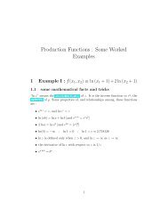
PORTFOLIO SELECTION Trading off expected return and risk ⢠How ...
PORTFOLIO SELECTION Trading off expected return and risk ⢠How ...
PORTFOLIO SELECTION Trading off expected return and risk ⢠How ...

Create successful ePaper yourself
Turn your PDF publications into a flip-book with our unique Google optimized e-Paper software.
Portfolio Selection 1<br />
<strong>PORTFOLIO</strong> <strong>SELECTION</strong><br />
<strong>Trading</strong> <strong>off</strong> <strong>expected</strong> <strong>return</strong> <strong>and</strong> <strong>risk</strong><br />
• <strong>How</strong> should we invest our wealth?<br />
Two principles:<br />
– we want to maximize <strong>expected</strong> <strong>return</strong><br />
– we want to minimize <strong>risk</strong> = variance
Portfolio Selection 2<br />
• goals somewhat at odds<br />
• <strong>risk</strong>ier assets generally have higher <strong>expected</strong> <strong>return</strong><br />
• investors dem<strong>and</strong> a reward for bearing <strong>risk</strong><br />
– called <strong>risk</strong> premium<br />
• there are optimal compromises between <strong>expected</strong><br />
<strong>return</strong> <strong>and</strong> <strong>risk</strong>
Portfolio Selection 3<br />
• In this chapter<br />
– maximize <strong>expected</strong> <strong>return</strong> with upper bound on<br />
the <strong>risk</strong><br />
– or minimize <strong>risk</strong> with lower bound on <strong>expected</strong><br />
<strong>return</strong>.
Portfolio Selection 4<br />
Key concept: reduction of <strong>risk</strong> by diversification<br />
• Diversification was not always considered favorably in<br />
the past
Portfolio Selection 5<br />
The investment philosophy of Keynes<br />
John Maynard Keynes wrote:<br />
... the management of stock exchange investment<br />
of any kind is a low pursuit ... from which it is a<br />
good thing for most members of society to be free<br />
I am in favor of having as large a unit as<br />
market conditions will allow ... to suppose<br />
that safety-first consists in having a small gamble<br />
in a large number of different [companies] where I<br />
have no information to reach a good judgement,<br />
as compared with a substantial stake in a<br />
company where ones’s information is adequate,<br />
strikes me as a travesty of investment policy
Portfolio Selection 6<br />
• Keynes is advocating stock picking or “fundamental<br />
analysis.”<br />
• semi-strong version of the EMH ⇒ fundamental<br />
analysis does not lead to profit<br />
• Keynes lived before the EMH<br />
– what Keynes would think about diversification<br />
now?<br />
• modern portfolio theory takes different view
Portfolio Selection 7<br />
• this is not to say that Keynes was wrong, but<br />
– Keynes was investing on a long time horizon<br />
– portfolio managers are judged on short-term<br />
successe<br />
– finding bargains is probably more difficult now
Portfolio Selection 8<br />
One <strong>risk</strong>y asset <strong>and</strong> one <strong>risk</strong>-free asset<br />
Start with a simple example:<br />
• one <strong>risk</strong>y asset, which could be a portfolio, e.g., a<br />
mutual fund<br />
– <strong>expected</strong> <strong>return</strong> is .15<br />
– st<strong>and</strong>ard deviation of the <strong>return</strong> is .25<br />
• one <strong>risk</strong>-free asset, e.g., a 30-day T-bill<br />
– <strong>expected</strong> value of the <strong>return</strong> is .06<br />
– st<strong>and</strong>ard deviation of the <strong>return</strong> is 0 by definition<br />
of “<strong>risk</strong>-free.”
Portfolio Selection 9<br />
Problem: construct an investment portfolio<br />
• a fraction w of our wealth is invested in the <strong>risk</strong>y asset<br />
• the remaining fraction 1 − w is invested in the<br />
<strong>risk</strong>-free asset<br />
• then the <strong>expected</strong> <strong>return</strong> is<br />
E(R) = w(.15) + (1 − w)(.06) = .06 + .09w.<br />
• the variance of the <strong>return</strong> is<br />
σ 2 R = w 2 (.25) 2 + (1 − w) 2 (0) 2 = w 2 (.25) 2 .<br />
<strong>and</strong> the st<strong>and</strong>ard deviation of the <strong>return</strong> is<br />
σ R = .25 w.<br />
Would w > 1 make any sense?
Portfolio Selection 10<br />
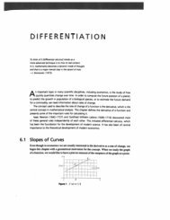
"Reward" = E(R) = .06+.09w<br />
0.2<br />
0.18<br />
0.16<br />
0.14<br />
0.12<br />
0.1<br />
0.08<br />
0.06<br />
0.04<br />
0.02<br />
0<br />
0 0.05 0.1 0.15 0.2 0.25<br />
"Risk" = σ R<br />
= w/4<br />
Plotting the portfolios in “reward-<strong>risk</strong> space”
Portfolio Selection 11<br />
• need to choose w:<br />
– choose the <strong>expected</strong> <strong>return</strong> E(R) , or<br />
– the amount of <strong>risk</strong> σ R<br />
• Once either E(R) or σ R is chosen, w can be<br />
determined.
Portfolio Selection 12<br />
Question: Suppose you want an <strong>expected</strong> <strong>return</strong> of .10?<br />
What should w be?<br />
Answer: .10 = .06 + .09 w ⇒ w = 4/9<br />
Question: Suppose you want σ R = .05. What should w<br />
be?<br />
Answer: .05 = w(.25) ⇒ w = 0.2
Portfolio Selection 13<br />
• More generally, if<br />
– the <strong>expected</strong> <strong>return</strong>s on the <strong>risk</strong>y <strong>and</strong> <strong>risk</strong>-free<br />
assets are µ 1 <strong>and</strong> µ f<br />
– <strong>and</strong> the st<strong>and</strong>ard deviation of the <strong>risk</strong>y asset is σ 1 ,<br />
• then<br />
– the <strong>expected</strong> <strong>return</strong> on the portfolio is<br />
wµ 1 + (1 − w)µ f<br />
– <strong>and</strong> the st<strong>and</strong>ard deviation of the portfolio’s <strong>return</strong><br />
is w σ 1 .
Portfolio Selection 14<br />
• This model of one <strong>risk</strong>-free asset <strong>and</strong> one <strong>risk</strong>y asset<br />
is simple but not useless<br />
• finding an optimal portfolio can be achieved in two<br />
steps.<br />
1. finding the “optimal” portfolio of <strong>risk</strong>y assets,<br />
called the tangency portfolio<br />
2. finding the appropriate mix of the <strong>risk</strong>-free asset<br />
<strong>and</strong> the tangency portfolio determined in step one<br />
• So we now know how to do the second step.<br />
• What we need to learn is how to mix optimally a<br />
number of <strong>risk</strong>y assets<br />
• First, we look at a related example.
Portfolio Selection 15<br />
Example<br />
• From February 2001 issue of PaineWebber’s<br />
Investment Intelligence: A Report for Our Clients<br />
• advantages of holding municipal bonds are touted<br />
• PaineWebber: “The chart at the right shows that a<br />
20% municipal/80% S&P 500 mix<br />
– sacrificed only 0.42% annual after-tax <strong>return</strong><br />
relative to a 100% S&P 500 portfolio<br />
– while reducing <strong>risk</strong> by 13.6% from 14.91% to<br />
12.88%.
Portfolio Selection 16<br />
• PaineWebber’s point is correct<br />
• but chart is cleverly designed to over-emphasize the<br />
reduction in volatility; how?
Portfolio Selection 17<br />
Estimating E(R) <strong>and</strong> σ R<br />
• <strong>risk</strong>-free rate, µ f , will be known<br />
– Treasury bill rates are published in most<br />
newspapers <strong>and</strong> web sites providing financial<br />
information.<br />
• what should we use as the values of E(R) <strong>and</strong> σ R ?<br />
• if <strong>return</strong>s on the asset are stationary<br />
– then can take past <strong>return</strong>s <strong>and</strong> use sample mean<br />
<strong>and</strong> st<strong>and</strong>ard deviation
Portfolio Selection 18<br />
• stationarity assumption is debatable.<br />
• E(R) <strong>and</strong> σ R could be adjusted subjectively<br />
• related question: how long a time series to use<br />
• long series, say 10 or 20 years, give less variable<br />
estimates<br />
• shorter series (maybe 1 or 2 years) may be more<br />
representative of future.<br />
– but difficult to estimate <strong>expected</strong> <strong>return</strong>s with<br />
accuracy
Portfolio Selection 19<br />
Two <strong>risk</strong>y assets<br />
Risk versus <strong>expected</strong> <strong>return</strong><br />
• two <strong>risk</strong>y assets have <strong>return</strong>s R 1 <strong>and</strong> R 2<br />
• mix them in proportions w <strong>and</strong> 1 − w<br />
• the <strong>return</strong> is R = wR 1 + (1 − w)R 2<br />
• <strong>expected</strong> <strong>return</strong> on the portfolio is<br />
E(R) = wµ 1 + (1 − w)µ 2 = µ 2 + w(µ 1 − µ 2 )<br />
• let ρ 12 be the correlation so that σ R1 ,R 2<br />
= ρ 12 σ 1 σ 2 .<br />
• the variance of the <strong>return</strong> on the portfolio is<br />
σ 2 R = w 2 σ 2 1 + (1 − w) 2 σ 2 2 + 2w(1 − w)ρ 12 σ 1 σ 2 .
Portfolio Selection 20<br />
Example:<br />
If µ 1 = .14, µ 2 = .08, σ 1 = .2, σ 2 = .15, <strong>and</strong> ρ 12 = 0, then<br />
E(R) = µ 2 + w(µ 1 − µ 2 ) = .08 + .06w.<br />
Also, because ρ 12 = 0 in this example<br />
σ 2 R = w 2 σ 2 1 + (1 − w) 2 σ 2 2 + 2w(1 − w)ρ 12 σ 1 σ 2 .<br />
= (.2) 2 w 2 + (.15) 2 (1 − w) 2 .<br />
Using calculus, one can show that the portfolio with the<br />
minimum <strong>risk</strong> is<br />
w = .045/.125 = .36.
Portfolio Selection 21<br />
For this portfolio E(R) = .08 + (.06)(.36) = .1016 <strong>and</strong><br />
σ R = √ (.2) 2 (.36) 2 + (.15) 2 (.64) 2 = .12.
Portfolio Selection 22<br />
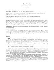
Here are values of E(R) <strong>and</strong> σ R for some other values of<br />
w:<br />
w E(R) σ R<br />
0 .080 .150<br />
1/4 .095 .123<br />
1/2 .110 .125<br />
3/4 .125 .155<br />
1 .140 .200
Portfolio Selection 23<br />
"Reward" = E(R)<br />
0.125<br />
0.1<br />
0.075<br />
F<br />
Efficient frontier −−><br />
T<br />
R1<br />
typical portfolio<br />
minimum variance portfolio<br />
R2<br />
0.05<br />
0 0.05 0.1 0.15 0.2 0.25 0.3<br />
"Risk" = σ R
Portfolio Selection 24<br />
Estimating means, st<strong>and</strong>ard deviations, <strong>and</strong><br />
covariances<br />
• estimates of µ 1 <strong>and</strong> σ 1 can be obtained from past<br />
<strong>return</strong>s on first <strong>risk</strong>y asset<br />
• denote this time series by R 1,1 , . . . , R 1,n<br />
• Let R 1 <strong>and</strong> s R1 be the sample mean <strong>and</strong> st<strong>and</strong>ard<br />
deviation of this series.<br />
• Similarly, µ 2 <strong>and</strong> σ 2 can be estimated from past<br />
<strong>return</strong>s on the second <strong>risk</strong>y asset
Portfolio Selection 25<br />
• The covariance σ 12 can be estimated by sample<br />
covariance<br />
n∑<br />
s 12 = n −1 (R 1,t − R 1 )(R 2,t − R 2 ).<br />
t=1<br />
• correlation ρ 12 can be estimated by the sample<br />
correlation<br />
̂ρ 12 = s 12<br />
s 1 s 2<br />
.
Portfolio Selection 26<br />
• Sample correlations <strong>and</strong> covariances can be computed<br />
PROC CORR in SAS<br />
• other estimates based on the CAPM will be<br />
introduced later
Portfolio Selection 27<br />
Combining two <strong>risk</strong>y assets with a <strong>risk</strong>-free asset<br />
Tangency portfolio with two <strong>risk</strong>y assets<br />
• each point on the efficient frontier is (σ R , E(R)) for<br />
some value of w<br />
• if we fix w, then we have a fixed portfolio of the two<br />
<strong>risk</strong>y assets.<br />
• Now let us mix that portfolio of <strong>risk</strong>y assets with the<br />
<strong>risk</strong>-free asset.
Portfolio Selection 28<br />
"Reward" = E(R)<br />
0.125<br />
0.1<br />
0.075<br />
F<br />
Efficient frontier −−><br />
T<br />
R1<br />
typical portfolio<br />
minimum variance portfolio<br />
R2<br />
0.05<br />
0 0.05 0.1 0.15 0.2 0.25 0.3<br />
"Risk" = σ R
Portfolio Selection 29<br />
• the slope of the line connecting the <strong>risk</strong>-free with a<br />
portfolio of <strong>risk</strong>ies is called the Sharpe ratio<br />
• Sharpe’s ratio = “reward-to-<strong>risk</strong>” ratio = ratio of<br />
“excess <strong>expected</strong> <strong>return</strong>” to st<strong>and</strong>ard deviation<br />
• the bigger the Sharpe ratio the better<br />
• The point T has highest Sharpe ratio <strong>and</strong> is called<br />
the tangency portfolio
Portfolio Selection 30<br />
Key result: “efficient” portfolios mix the tangency<br />
portfolio with the <strong>risk</strong>-free asset.<br />
• all efficient portfolios use the same mix of the<br />
two <strong>risk</strong>y assets, namely the tangency portfolio
Portfolio Selection 31<br />
Finding the tangency portfolio<br />
Define<br />
• V 1 = µ 1 − µ f<br />
• V 2 = µ 2 − µ f<br />
• V 1 <strong>and</strong> V 2 are called the “excess <strong>return</strong>s.”<br />
w T =<br />
V 1 σ 2 2 − V 2 ρ 12 σ 1 σ 2<br />
V 1 σ 2 2 + V 2 σ 2 1 − (V 1 + V 2 )ρ 12 σ 1 σ 2<br />
.
Portfolio Selection 32<br />
The tangency portfolio allocates:<br />
• w T to the first <strong>risk</strong>y asset<br />
• (1 − w T ) to the second <strong>risk</strong>y asset<br />
Notation: Let<br />
• R T = <strong>return</strong><br />
• E(R T ) = <strong>expected</strong> <strong>return</strong><br />
• σ T = st<strong>and</strong>ard deviation of the <strong>return</strong><br />
on the tangency portfolio.
Portfolio Selection 33<br />
Example:<br />
• as before µ 1 = .14, µ 2 = .08, σ 1 = .2, σ 2 = .15, <strong>and</strong><br />
ρ 12 = 0<br />
• suppose as well that µ f = .06<br />
• V 1 = .14 − .06 = .08<br />
• V 2 = .08 − .06 = .02.<br />
• Plugging into formula: w T = .693<br />
• Therefore,<br />
E(R T ) = (.693)(.14) + (.307)(.08) = .122,<br />
σ T = √ (.693) 2 (.2) 2 + (.307) 2 (.15) 2 = .146.
Portfolio Selection 34<br />
Let R be the <strong>return</strong> on the portfolio that allocates:<br />
• ω to the tangency portfolio<br />
• 1 − ω to the <strong>risk</strong>-free asset<br />
Then<br />
R = ωR T + (1 − ω)µ f<br />
= µ f + ω(R T − R f )<br />
E(R) = µ f + ω{E(R T ) − µ f }<br />
σ R = ωσ T .
Portfolio Selection 35<br />
Continuation of previous example: What is the<br />
optimal investment with σ R = .05?<br />
Answer:<br />
Since<br />
<strong>and</strong><br />
so that<br />
σ R = ωσ T .<br />
σ T = .146<br />
.05 = σ R = ω σ T = .146 ω<br />
ω = .05/.146 = .343 <strong>and</strong> 1 − ω = .657
Portfolio Selection 36<br />
• So 65.7% of the portfolio should be in the <strong>risk</strong>-free<br />
asset.<br />
• 34.3% should be in the tangency portfolio.<br />
• Thus (.343)(69.3%) = 23.7% should be in the first<br />
<strong>risk</strong>y asset<br />
• (.343)(30.7%) = 10.5 should be in the second <strong>risk</strong>y<br />
asset.
Portfolio Selection 37<br />
Asset Allocation<br />
<strong>risk</strong>-free 65.7%<br />
<strong>risk</strong>y 1 23.7%<br />
<strong>risk</strong>y 2 10.5%<br />
Total 99.9%
Portfolio Selection 38<br />
Now suppose that you want a 10% <strong>expected</strong> <strong>return</strong>.<br />
Compare<br />
• The best portfolio of only <strong>risk</strong>y assets<br />
• the best portfolio of the <strong>risk</strong>y assets <strong>and</strong> the <strong>risk</strong>-free<br />
asset<br />
Answer:<br />
• (best portfolio of <strong>risk</strong>y assets)<br />
* .1 = wµ 1 + (1 − w)µ 2 = w(.14) + (1 − w)(.08)<br />
= .08 + (.14 − .08)w<br />
* or w = (.1 − .08)/(.14 − .08) = .02/.06 = 1/3.<br />
* This is the only portfolio of <strong>risk</strong>y assets with<br />
E(R) = .1, so by default it is best.
Portfolio Selection 39<br />
• Then<br />
σ R =<br />
√<br />
w 2 σ 2 1 + (1 − w) 2 σ 2 2 = √ w 2 (.2) 2 + (1 − w) 2 (.15) 2<br />
= √ (1/9)(.2) 2 + 4/9(.15) 2 = .120.<br />
• (best portfolio of the two <strong>risk</strong>y assets <strong>and</strong> the <strong>risk</strong>-free<br />
asset)<br />
* .1 = E(R) = .06 + .062ω = .06 + .425σ R<br />
* This implies that σ R = .04/.425 = .094<br />
* σ R = ωσ T<br />
* or ω = σ R /σ T = .094/.146 = .644.
Portfolio Selection 40<br />
• combining the <strong>risk</strong>-free asset with the two <strong>risk</strong>y assets<br />
reduces σ R from .120 to .094 while maintaining E(R)<br />
at .1.<br />
• The reduction in <strong>risk</strong> is (.120 − .094)/.094 = 28%.<br />
• Not a bad reduction in <strong>risk</strong>!
Portfolio Selection 41<br />
More on the example: What is the best we can do<br />
combining the <strong>risk</strong>-free asset with only one <strong>risk</strong>y asset?<br />
Assume that we still want to have E(R) = .1<br />
• Second <strong>risk</strong>y asset with the <strong>risk</strong>-free<br />
– Since µ f = .06 < .1 <strong>and</strong> µ 2 = .08 < .1, no portfolio<br />
with only the second <strong>risk</strong>y asset <strong>and</strong> the <strong>risk</strong>-free<br />
asset will have an <strong>expected</strong> <strong>return</strong> of .1.<br />
– Another way to appreciate this fact is to solve<br />
.1 = ω(.08) + (1 − ω)(.06) = .06 + .02ω<br />
to get ω = 2 <strong>and</strong> 1 − ω = −1.
Portfolio Selection 42<br />
• <strong>How</strong>ever, ω <strong>and</strong> 1 − ω must both be between 0 <strong>and</strong> 1<br />
unless one is permitted to sell short or buy on margin<br />
• Selling short means selling an asset one does not yet<br />
owe <strong>and</strong> purchasing it later at delivery time.<br />
• First <strong>risk</strong>y asset with the <strong>risk</strong>-free<br />
* .1 = ω(.14) + (1 − ω)(.06) = .06 + ω(.08) imples<br />
that ω = .04/.08 = 1/2.<br />
* Then σ R = ω(.20) = .10 which is greater than .094
Portfolio Selection 43<br />
The minimum value of σ R under various combinations of<br />
available assets (E(R) fixed at .1):<br />
Available Assets<br />
Minimum σ R<br />
1st <strong>risk</strong>y <strong>and</strong> <strong>risk</strong>-free 0.1<br />
2nd <strong>risk</strong>y <strong>and</strong> <strong>risk</strong>-free –<br />
Both <strong>risk</strong>ies, but no <strong>risk</strong>-free 0.12<br />
All three 0.094
Portfolio Selection 44<br />
Effect of ρ 12<br />
• Correlation effects only the <strong>risk</strong>, not the <strong>expected</strong><br />
<strong>return</strong>.<br />
• Positive correlation between the two <strong>risk</strong>y asets is<br />
bad.<br />
• With positive correlation, the two assets tend to move<br />
together which increases the volatility of the portfolio.<br />
• Conversely, negative correlation is good.<br />
• If the assets are negatively correlated, a negative<br />
<strong>return</strong> of one tends to occur with a positive <strong>return</strong> of<br />
the other
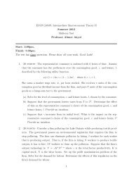
Portfolio Selection 45<br />
• Figure shows the efficient frontier <strong>and</strong> tangency<br />
portfolio when µ 1 = .14, µ 2 = .09, σ 1 = .2, σ 2 = .15,<br />
<strong>and</strong> µ f = .03.<br />
• The value of ρ 12 is varied from .7 to −.7.<br />
• The Sharpe’s ratio of the tangency portfolio <strong>return</strong>s<br />
increases as ρ 12 decreases.
Portfolio Selection 46<br />
0.1<br />
ρ = 0.7<br />
T<br />
*<br />
0.1<br />
ρ = 0.3<br />
T<br />
*<br />
E(R)<br />
E(R)<br />
0.05<br />
F<br />
*<br />
0 0.05 0.1 0.15 0.2<br />
σ R<br />
ρ = 0<br />
0.05<br />
F<br />
*<br />
0 0.05 0.1 0.15 0.2<br />
σ R<br />
ρ = −0.7<br />
0.1<br />
T<br />
*<br />
0.1<br />
T<br />
*<br />
E(R)<br />
E(R)<br />
0.05<br />
F<br />
*<br />
0 0.05 0.1 0.15 0.2<br />
σ R<br />
0.05<br />
F<br />
*<br />
0 0.05 0.1 0.15 0.2<br />
σ R
Portfolio Selection 47<br />
Risk-efficient portfolios with N <strong>risk</strong>y assets<br />
Efficient-set mathematics<br />
Efficient-set mathematics generalizes our previous<br />
analysis with two <strong>risk</strong>y assets to the more realistic case of<br />
many <strong>risk</strong>y assets. This material is taken from<br />
Section 5.2 of Campbell, Lo, <strong>and</strong> MacKinlay.
Portfolio Selection 48<br />
Assume that we have N <strong>risk</strong>y assets <strong>and</strong> that the <strong>return</strong><br />
on the ith <strong>risk</strong>y asset is µ i . Define<br />
⎛ ⎞<br />
R 1<br />
R = ⎝ . ⎠<br />
R N<br />
to be the r<strong>and</strong>om vector of <strong>return</strong>s. Then<br />
⎛ ⎞<br />
µ 1<br />
E(R) = µ = ⎝ . ⎠ .<br />
µ N
Portfolio Selection 49<br />
• Let Ω ij be the covariance between R i <strong>and</strong> R j .<br />
• Also, let σ i = √ Ω ii be the the st<strong>and</strong>ard deviation of<br />
R i .<br />
• Define ρ ij = Ω ij /(σ i σ j ) as the correlation between R i<br />
<strong>and</strong> R j .<br />
• Finally, let Ω be the covariance matrix of R, i.e.,<br />
Ω = COV(R),<br />
– so that the i, jth element of Ω is Ω ij = Cov(R i , R j ).
Portfolio Selection 50<br />
• Let<br />
⎛<br />
ω = ⎝<br />
⎞<br />
ω 1<br />
. ⎠<br />
ω N<br />
be a matrix of portfolio weights <strong>and</strong><br />
• let<br />
⎛<br />
⎞<br />
1 =<br />
⎝<br />
1.<br />
1<br />
be a column of N ones. (Use to simplify notation.)<br />
⎠
Portfolio Selection 51<br />
With this notation, we can now write down the problem<br />
succinctly.<br />
• We assume that ω 1 + · · · + ω N = 1 T ω = 1.<br />
• The <strong>expected</strong> <strong>return</strong> on a portfolio with weights ω is<br />
N∑<br />
ω i µ i = ω T µ.<br />
i=1
Portfolio Selection 52<br />
• Suppose there is a target value, µ P , of the <strong>expected</strong><br />
<strong>return</strong> on the portfolio.<br />
• When N = 2 the target, µ P , is achieved by only one<br />
portfolio <strong>and</strong> its ω 1 value solves<br />
µ P = ω 1 µ 1 + ω 2 µ 2 = µ 2 + ω 1 (µ 1 − µ 2 ).
Portfolio Selection 53<br />
• For N ≥ 3, there will be an infinite number of<br />
portfolios achieving the target, µ P .<br />
• The one with the smallest variance is called the<br />
“efficient” portfolio.<br />
• Our goal is to find the efficient portfolio.
Portfolio Selection 54<br />
The variance of the <strong>return</strong> on the portfolio with weights<br />
ω is<br />
N∑ N∑<br />
ω i ω j Ω ij = ω T Ωω. (1)<br />
i=1<br />
j=1<br />
Thus, given a target µ P , the efficent portfolio minimizes<br />
(1) subject to<br />
<strong>and</strong><br />
ω T µ = µ P (2)<br />
ω T 1 = 1. (3)<br />
• This is a quadratic programming (QP) problem.<br />
• QP also allows us to impose the constraints ω i ≥ 0.<br />
– Later
Portfolio Selection 55<br />
We will denote the weights of the efficient portfolio by<br />
ω µP . To find ω µP , form the Lagrangian<br />
Then solve<br />
L = ω T Ωω + δ 1 (µ P − ω T µ P<br />
µ) + δ 2 (1 − ω T 1).<br />
0 = ∂<br />
∂ω L = 2Ωω µ P<br />
− δ 1 µ − δ 2 1. (4)<br />
Now we will look at the details of the derivation of (4).
Portfolio Selection 56<br />
Definition: Here<br />
⎛<br />
∂<br />
∂ω L = ⎜<br />
⎝<br />
⎞<br />
∂ L/∂ ω 1<br />
⎟<br />
. ⎠<br />
∂ L/∂ ω N<br />
means the gradient of L with respect to ω with the other<br />
variables in L held fixed.
Portfolio Selection 57<br />
Fact: For an n × n matrix A <strong>and</strong> an n-dimensional<br />
vector x,<br />
∂<br />
∂x xT Ax = (A + A T )x<br />
(This gives us the first term in (4).)<br />
The solution to (4) is<br />
ω µP = 1 2 Ω−1 (δ 1 µ + δ 2 1) = Ω −1 (λ 1 µ + λ 2 1)<br />
where λ 1 <strong>and</strong> λ 2 are new Lagrange multipliers:<br />
λ 1 = 1 2 δ 1 <strong>and</strong> λ 2 = 1 2 δ 2.
Portfolio Selection 58<br />
Thus,<br />
ω µP = λ 1 Ω −1 µ + λ 2 Ω −1 1,<br />
where λ 1 <strong>and</strong> λ 2 are yet to be determined scalar<br />
quantities. We need to use the constraints to determine<br />
λ 1 <strong>and</strong> λ 2 . Therefore,<br />
µ p = µ T ω µP = λ 1 µ T Ω −1 µ + λ 2 µ T Ω −1 1, (5)<br />
<strong>and</strong><br />
1 = 1 T ω µP = λ 1 1 T Ω −1 µ + λ 2 1 T Ω −1 1. (6)
Portfolio Selection 59<br />
These are equations in λ 1 <strong>and</strong> λ 2 . We will introduce<br />
simpler notation for the coefficients:<br />
A = µ T Ω −1 1 = 1 T Ω −1 µ<br />
B = µ T Ω −1 µ,<br />
C = 1 T Ω −1 1.<br />
Then (5) <strong>and</strong> (6) can be rewritten as<br />
µ P = Bλ 1 + Aλ 2<br />
1 = Aλ 1 + Cλ 2 .<br />
Let D = BC − A 2 be the determinant of this system of<br />
linear equations. The solution is<br />
λ 1 = −A + C µ p<br />
D<br />
<strong>and</strong> λ 2 = B − A µ P<br />
D<br />
.
Portfolio Selection 60<br />
It follows after some algebra that<br />
where<br />
<strong>and</strong><br />
ω µP = g + h µ P , (7)<br />
g = B Ω−1 1 − A Ω −1 µ<br />
, (8)<br />
D<br />
h = C Ω−1 µ − A Ω −1 1<br />
. (9)<br />
D<br />
Notice that g <strong>and</strong> h are fixed vectors, since they depend<br />
on the fixed vector µ <strong>and</strong> the fixed matrix Ω. Also, the<br />
scalars A, C, <strong>and</strong> D are functions of µ <strong>and</strong> Ω so they are<br />
also fixed.
Portfolio Selection 61<br />
The target <strong>expected</strong> <strong>return</strong>, µ P , can be varied over the<br />
range<br />
min µ i ≤ µ P ≤ max µ i.<br />
i=1,...,N i=1,...,N<br />
As µ P varies over this range, we get a locus ω µP of<br />
efficient portfolios called the “efficient frontier.” We can<br />
illustrate the efficient frontier by the following algorithm:<br />
1. Vary µ P along a grid. For each value of µ P on this<br />
grid, compute σ µP by:<br />
(a) computing ω µP = g + h µ P<br />
√<br />
(b) then computing σ µP = ω T µ P<br />
Ωω µP<br />
2. Plot the values (µ P , σ µP )
Portfolio Selection 62<br />
This algorithm is implemented in the MATLAB program<br />
“portfolio02.m” listed below:<br />
bmu = [.08;.03;.05] ;<br />
bOmega = [ .3 .02 .01 ;<br />
.02 .15 .03 ;<br />
.01 .03 .18 ] ;<br />
bone = ones(length(bmu),1) ;<br />
ngrid = 200 ;<br />
muP = linspace(-.02,.2,ngrid) ;<br />
sigmaP = zeros(1,ngrid) ;<br />
omegaP = zeros(length(bmu),ngrid) ;<br />
mu12 = zeros(1,ngrid) ;<br />
sigma12 = mu12 ;<br />
mu13 = zeros(1,ngrid) ;<br />
sigma13 = mu12 ;<br />
mu23 = zeros(1,ngrid) ;<br />
sigma23 = mu12 ;
Portfolio Selection 63<br />
ibOmega = inv(bOmega) ;<br />
A = bone’*ibOmega*bmu ;<br />
B = bmu’*ibOmega*bmu ;<br />
C = bone’*ibOmega*bone ;<br />
D = B*C - A^2 ;<br />
bg = (B*ibOmega*bone - A*ibOmega*bmu)/D ;<br />
bh = (C*ibOmega*bmu - A*ibOmega*bone)/D
Portfolio Selection 64<br />
for i=1:ngrid ;<br />
omegaP(:,i) = bg + muP(i)*bh ;<br />
sigmaP(i) = sqrt(omegaP(:,i)’*bOmega*omegaP(:,i)) ;<br />
mu12(i) = w(i)*bmu(1) + (1-w(i))*bmu(2) ;<br />
sigma12(i) = sqrt(w(i)^2*bOmega(1,1) + 2*w(i)*(1-w(i))*bOmega(1,2) ...<br />
+ (1-w(i))^2*bOmega(2,2)) ;<br />
mu13(i) = w(i)*bmu(1) + (1-w(i))*bmu(3) ;<br />
sigma13(i) = sqrt(w(i)^2*bOmega(1,1) + 2*w(i)*(1-w(i))*bOmega(1,3) ...<br />
+ (1-w(i))^2*bOmega(3,3)) ;<br />
mu23(i) = w(i)*bmu(2) + (1-w(i))*bmu(3) ;<br />
sigma23(i) = sqrt(w(i)^2*bOmega(2,2) + 2*w(i)*(1-w(i))*bOmega(2,3) ...<br />
+ (1-w(i))^2*bOmega(3,3))<br />
end ;
Portfolio Selection 65<br />
fsize = 16 ;<br />
figure(1)<br />
p = plot(sigmaP,muP,sigma12,mu12,’--’,sigma13,mu13, ...<br />
’-.’,sigma23,mu23,’:’) ;<br />
set(p,’linewidth’,6) ;<br />
xlabel(’st<strong>and</strong>ard deviation of <strong>return</strong> (\sigma_P)’,’fontsize’,fsize) ;<br />
ylabel(’<strong>expected</strong> <strong>return</strong> (\mu_P)’,’fontsize’,fsize) ;<br />
text(sqrt(bOmega(1,1)),bmu(1),’1’,’fontsize’,24) ;<br />
text(sqrt(bOmega(2,2)),bmu(2),’2’,’fontsize’,24) ;<br />
text(sqrt(bOmega(3,3)),bmu(3),’3’,’fontsize’,24) ;<br />
set(gca,’fontsize’,fsize) ;<br />
set(gca,’ylim’,[-.02,.2]) ;<br />
set(gca,’xlim’,[.2,2]) ; end ;<br />
print portfolio02SH.ps -depsc ;
Portfolio Selection 66<br />
figure(2)<br />
p2 = plot(muP,omegaP(1,:),muP,omegaP(2,:),’--’,muP,omegaP(3,:),’-.’) ;<br />
set(p2,’linewidth’,6) ;<br />
set(gca,’fontsize’,fsize) ;<br />
grid ;<br />
xlabel(’\mu_P’,’fontsize’,fsize) ;<br />
ylabel(’weight’,’fontsize’,fsize) ;<br />
legend(’w_1’,’w_2’,’w_3’,0) ;<br />
print portfolio02.ps -depsc ;
Portfolio Selection 67<br />
0.08<br />
1<br />
0.07<br />
<strong>expected</strong> <strong>return</strong> (µ P<br />
)<br />
0.06<br />
0.05<br />
0.04<br />
3<br />
0.03<br />
2<br />
0.25 0.3 0.35 0.4 0.45 0.5 0.55 0.6<br />
st<strong>and</strong>ard deviation of <strong>return</strong> (σ P<br />
)<br />
From portfolio02.m
Portfolio Selection 68<br />
1<br />
0.8<br />
0.6<br />
weight<br />
0.4<br />
0.2<br />
0<br />
w 1<br />
w 2<br />
w 3<br />
−0.2<br />
−0.4<br />
0.045 0.05 0.055 0.06 0.065 0.07 0.075 0.08<br />
µ P<br />
From portfolio02.m
Portfolio Selection 69<br />
• If one wants to avoid short selling, then one must<br />
impose the additional constraints that w i ≥ 0 for<br />
i = 1, . . . , N.<br />
• Minimization of portfolio <strong>risk</strong> subject to ω T µ = µ P ,<br />
ω T 1 = 1, <strong>and</strong> these additional nonnegativity<br />
constraints is a quadratic programming problem.<br />
• The program “quadprog” in MATLAB’s<br />
Optimization Toolbox does quadratic programming.<br />
• Figures were produced by the program<br />
“portfolio02QP.m” that uses “quadprog” in<br />
MATLAB.
Portfolio Selection 70<br />
0.08<br />
1<br />
0.07<br />
<strong>expected</strong> <strong>return</strong> (µ P<br />
)<br />
0.06<br />
0.05<br />
0.04<br />
3<br />
0.03<br />
2<br />
no negative wts<br />
unconstrained wts<br />
0.25 0.3 0.35 0.4 0.45 0.5 0.55 0.6<br />
st<strong>and</strong>ard deviation of <strong>return</strong> (σ P<br />
)<br />
From portfolio02QP.m
Portfolio Selection 71<br />
1<br />
w 1<br />
w 2<br />
w 3<br />
From portfolio02QP.m<br />
weight<br />
0.5<br />
0<br />
0.045 0.05 0.055 0.06 0.065 0.07 0.075 0.08<br />
µ P
Portfolio Selection 72<br />
• Now suppose that we have a <strong>risk</strong>-free asset <strong>and</strong> we<br />
want to mix the <strong>risk</strong>-free asset with some efficient<br />
portfolio.<br />
• One can see geometrically that there is a tangency<br />
portfolio; see the figure.<br />
• The optimal portfolio always is a mixture of<br />
the <strong>risk</strong>-free asset with the tangency portfolio.<br />
• This is a remarkable simplification.
Portfolio Selection 73
Portfolio Selection 74<br />
Selling short<br />
• Selling short is a way to profit if a stock price goes<br />
down.<br />
• To sell a stock short, one sells the stock without<br />
owning it.<br />
• Suppose a stock is selling at $25/share <strong>and</strong> you sell<br />
100 shares short.<br />
– This gives you $2,500.<br />
– If the goes down to $17 share, you can buy the 100<br />
shares for $1,700 <strong>and</strong> close out your short position.
Portfolio Selection 75<br />
• Suppose that you have $100 <strong>and</strong> there are two <strong>risk</strong>y<br />
assets.<br />
• With your money you could buy<br />
– $150 worth of <strong>risk</strong>y asset 1 <strong>and</strong><br />
– sell $50 short of <strong>risk</strong>y asset 2.<br />
• the net cost would be exactly $100.<br />
• the <strong>return</strong> on your portfolio would be<br />
(<br />
3<br />
2 R 1 + − 1 )<br />
R 2 .<br />
2<br />
• Your portfolio weights are w 1 = 3/2 <strong>and</strong> w 2 = −1/2.<br />
Values of µ P below min(µ i ) <strong>and</strong> above max(µ i ) are<br />
possible by using short selling.
Portfolio Selection 76<br />
The Interior decorator fallacy<br />
• It is often thought that a stock portfolio should be<br />
tailored to the financial circumstances of a client.<br />
• Bernstein, in Capital Ideas, calls this the “interior<br />
decorator fallacy.”
Portfolio Selection 77<br />
• Example: a woman in her forties married to a<br />
clergyman with a modest income.<br />
• inherited money which she wanted to invest.<br />
Bernstein recommended stocks with good growth<br />
potential but low dividends, e.g., Georgia Pacific,<br />
IBM, <strong>and</strong> Gillette.<br />
• The client was worried that these were too <strong>risk</strong>y<br />
• Bernstein reasoned that even someone with modest<br />
means should benefit from the long-term growth<br />
potential
Portfolio Selection 78<br />
• Another Example: Bernstein recommended electric<br />
utilities, a conservative choice, to a young business<br />
excecutive who wanted a more aggressive portfolio.<br />
• Again, this recommendation was at odds with<br />
conventional wisdom.<br />
• New view: there is a best portfolio (the tangency<br />
portfolio) that is the same for everyone.<br />
• An individual’s circumstances only determines the<br />
appropriate mix between <strong>risk</strong>-free assets <strong>and</strong> the<br />
tangency portfolio. The clergyman’s wife should<br />
invest a higher percentage of her money
Portfolio Selection 79<br />
Back to the math – finding the tangency portfolio<br />
• Now remove the assumption that ω T 1 = 1.<br />
• The quantity 1 − ω T 1 is invested in the <strong>risk</strong>-free<br />
asset. (Does it make sense to have 1 − ω T 1 < 0?).<br />
• The <strong>expected</strong> <strong>return</strong> is<br />
ω T µ + (1 − ω T 1)µ f ,<br />
• The constraint is that <strong>expected</strong> <strong>return</strong> is equal to µ P .
Portfolio Selection 80<br />
• Thus, the Lagrangian function is<br />
• Since<br />
L = ω T Ωω + δ{µ P − ω T µ − (1 − ω T 1)µ f }.<br />
0 = ∂<br />
∂ ω L = 2Ωω + δ(−µ + 1µ f),<br />
the optimal weight vector is<br />
where λ = δ/2.<br />
ω µP = λΩ −1 (µ − µ f 1), (10)
Portfolio Selection 81<br />
• To find λ, we use our constraint:<br />
ω T µ P<br />
µ + (1 − ω T µ P<br />
1)µ f = µ P . (11)<br />
• Rearranging (11), we get<br />
ω T µ P<br />
(µ − µ f 1) = µ P − µ f . (12)<br />
• Therefore, substituting (10) into (12) we have<br />
λ(µ − µ f 1) T Ω −1 (µ − µ f 1) = µ P − µ f ,<br />
or<br />
λ =<br />
µ P − µ f<br />
(µ − µ f ) T Ω −1 (µ − µ f 1) . (13)
Portfolio Selection 82<br />
• Then substituting (13) into (10)<br />
ω µP = c P ω,<br />
where<br />
<strong>and</strong><br />
c P =<br />
µ P − µ f<br />
(µ − µ f 1) T Ω −1 (µ − µ f 1)<br />
ω = Ω −1 (µ − µ f 1). (14)<br />
• (µ − µ f 1) is the vector of “excess <strong>return</strong>s,” that is,<br />
the amount by which the <strong>expected</strong> <strong>return</strong>s on the<br />
<strong>risk</strong>y assets exceed the <strong>risk</strong>-free <strong>return</strong>.<br />
• The excess <strong>return</strong>s measure how much the market<br />
pays for assuming <strong>risk</strong>.
Portfolio Selection 83<br />
• ω is not quite a portfolio because these weights do<br />
not necessarily sum to one.<br />
• The tangency portfolio is a scalar multiple of ω:<br />
ω T =<br />
ω<br />
1 T ω . (15)<br />
• ω T is a portfolio since the weight are forced to sum to<br />
one.
Portfolio Selection 84<br />
• The optimal weight vector ω µP can be expressed in<br />
terms of the tangency portfolio as<br />
ω µP<br />
= c p ω = c p (1 T ω)ω T<br />
• Therefore, c P (1 T ω) tells us how much weight to put<br />
on the tangency portfolio, ω T .<br />
• The amount of weight to put of the <strong>risk</strong>-free asset is<br />
= 1 − c p (ω T 1).<br />
Note that ω <strong>and</strong> ω T do not depend on µ p .
Portfolio Selection 85<br />
• The MATLAB program “portfolio04.m” on the course<br />
web site is an extension of “portfolio02.m.”<br />
• portfolio04.m, which is listed below, also plots of<br />
– the tangency portfolio (T) <strong>and</strong><br />
– the line connecting the <strong>risk</strong>-free asset (F) with the<br />
tangency portfolio.<br />
• We’ll look at the plot first
Portfolio Selection 86<br />
0.08<br />
0.07<br />
<strong>expected</strong> <strong>return</strong><br />
0.06<br />
0.05<br />
0.04<br />
* T<br />
* P<br />
0.03<br />
F<br />
*<br />
0.02<br />
0 0.05 0.1 0.15 0.2 0.25 0.3 0.35 0.4 0.45 0.5<br />
st<strong>and</strong>ard deviation of <strong>return</strong><br />
Efficient frontier <strong>and</strong> tangency portfolio plotted<br />
by the program “portfolio04.m” for N = 3 assets.
Portfolio Selection 87<br />
Input data µ, Ω, <strong>and</strong> µ f . Create 1.<br />
bmu = [.08;.03;.05] ;<br />
bOmega = [ .3 .02 .01 ;<br />
.02 .15 .03 ;<br />
.01 .03 .18 ] ;<br />
muf = .02 ;<br />
bone = ones(length(bmu),1) ;
Portfolio Selection 88<br />
Create grid of µ P values <strong>and</strong> set up storage. Invert Ω.<br />
muP = linspace(min(bmu),max(bmu),50) ;<br />
sigmaP = zeros(1,50) ;<br />
ibOmega = inv(bOmega) ;
Portfolio Selection 89<br />
Create A, B, C, <strong>and</strong> D <strong>and</strong> also the vectors g <strong>and</strong> h.<br />
A = bone’*ibOmega*bmu ;<br />
B = bmu’*ibOmega*bmu ;<br />
C = bone’*ibOmega*bone ;<br />
D = B*C - A^2 ;<br />
bg = (B*ibOmega*bone - A*ibOmega*bmu)/D ;<br />
bh = (C*ibOmega*bmu - A*ibOmega*bone)/D ;
Portfolio Selection 90<br />
Compute ω <strong>and</strong> σ P for each target <strong>expected</strong> <strong>return</strong> on<br />
the portfolio.<br />
for i=1:50 ;<br />
end ;<br />
omegaP = bg + muP(i)*bh ;<br />
sigmaP(i) = sqrt(omegaP’*bOmega*omegaP) ;
Portfolio Selection 91<br />
Compute the minimum variance <strong>return</strong>.<br />
gg = bg’*bOmega*bg ;<br />
hh = bh’*bOmega*bh ;<br />
gh = bg’*bOmega*bh ;<br />
mumin = - gh/hh ;<br />
sdmin = sqrt( gg * ( 1 - gh^2/(gg*hh)) ) ;
Portfolio Selection 92<br />
Compute the tangency portfolio<br />
bomegabar = ibOmega*(bmu - muf*bone) ;<br />
bomegaT = bomegabar/(bone’*bomegabar) ;<br />
sigmaT = sqrt(bomegaT’*bOmega*bomegaT) ;<br />
muT = bmu’*bomegaT ;
Portfolio Selection 93<br />
Compute quantities needed for plotting. “P2” is a typical<br />
portfolio.<br />
fsize = 16 ;<br />
fsize2 = 35 ;<br />
bomegaP2 = [0;.3;.7] ;<br />
sigmaP2 = sqrt(bomegaP2’*bOmega*bomegaP2) ;<br />
muP2 = bmu’*bomegaP2 ;
Portfolio Selection 94<br />
Plot efficient frontier <strong>and</strong> line connecting the <strong>risk</strong>-free<br />
asset <strong>and</strong> the tangency portfolio.<br />
ind = (muP > mumin) ;<br />
% Indicates efficient horizon<br />
ind2 = (muP < mumin) ;<br />
% Indicates locus below efficient horizon<br />
p1 = plot(sigmaP(ind),muP(ind),’-’,sigmaP(ind2),muP(ind2),...<br />
’--’ ,sdmin,mumin,’.’) ;<br />
l1 = line([0,sigmaT],[muf,muT]) ;
Portfolio Selection 95<br />
Annotate the plot.<br />
t1= text(sigmaP2,muP2,’* P’,’fontsize’,fsize2) ;<br />
t2= text(sigmaT,muT,’* T’,’fontsize’,fsize2) ;<br />
t3=text(.01,muf+.006,’F’,’fontsize’,fsize2) ;<br />
t3B = text(0,muf,’*’,’fontsize’,fsize2) ;<br />
set(p1(1:2),’linewidth’,4) ;<br />
set(p1(3),’markersize’,40) ;<br />
set(p1(3),’color’,’red’) ;<br />
set(l1,’linewidth’,4) ;<br />
set(l1,’linestyle’,’--’) ;<br />
xlabel(’st<strong>and</strong>ard deviation of <strong>return</strong>’,’fontsize’,fsize) ;<br />
ylabel(’<strong>expected</strong> <strong>return</strong>’,’fontsize’,fsize) ;
Portfolio Selection 96<br />
Here’s the plot again.<br />
0.08<br />
0.07<br />
<strong>expected</strong> <strong>return</strong><br />
0.06<br />
0.05<br />
0.04<br />
* T<br />
* P<br />
0.03<br />
F<br />
*<br />
0.02<br />
0 0.05 0.1 0.15 0.2 0.25 0.3 0.35 0.4 0.45 0.5<br />
st<strong>and</strong>ard deviation of <strong>return</strong><br />
Efficient frontier <strong>and</strong> tangency portfolio plotted by the<br />
program “portfolio04.m” for N = 3 assets.
Portfolio Selection 97<br />
Is the theory useful?<br />
• This theory of portfolio selection could be used if N<br />
were small. We would need estimates of µ <strong>and</strong> Ω.<br />
• These would be obtained from recent <strong>return</strong>s data.<br />
• Working assumption – future <strong>return</strong>s will be similar<br />
to past <strong>return</strong>s<br />
• Another problem is that the results are very sensitive<br />
to estimation error<br />
– <strong>and</strong> <strong>expected</strong> <strong>return</strong>s are difficult to estimate<br />
accurately
Portfolio Selection 98<br />
• The next section gives an example of using portfolio<br />
theory to allocate capital among eight international<br />
markets.<br />
• With a total of only eight assets, implementing the<br />
theory is feasible.<br />
• <strong>How</strong>ever, suppose that we were considering selecting a<br />
portfolio from all 500 stocks on the S&P index.
Portfolio Selection 99<br />
• Or, even worse, consider all 3000 stocks on the<br />
Russell index. Ugh!<br />
– There would be (3000)(2999)/2 ≈ 4.5 million<br />
covariances to estimate.<br />
– Moreover, Ω would be 3000 by 3000 <strong>and</strong> its inverse<br />
is required.<br />
– most serious difficulty would not be the<br />
computations.<br />
∗ more difficult problems are costs of data<br />
collection <strong>and</strong> poor estimation accuracy
Portfolio Selection 100<br />
• Portfolio theory was an important theoretical<br />
development.<br />
– Markowitz was awarded the Nobel Prize in<br />
economics for this work.<br />
• <strong>How</strong>ever, a practical version of this theory awaited<br />
the work of Sharpe <strong>and</strong> Lintner.<br />
• Sharpe, who was Markowitz’s PhD student, shared<br />
the Nobel Prize with Markowitz.<br />
• Sharpe’s CAPM asserts that the tangency portfolio<br />
is also the market portfolio<br />
– This is a tremendous simplification.
Portfolio Selection 101<br />
Example—Global Asset Allocation<br />
• This example is taken from Efficient Asset<br />
Management by Richard O. Michaud.<br />
• The problem is to allocate capital to eight major<br />
classes of assets:<br />
– U.S. stocks<br />
– U.S. government <strong>and</strong> corporate bonds<br />
– Euros<br />
– the Canadian, French, German, Japanese, <strong>and</strong><br />
U.K. equity markets
Portfolio Selection 102<br />
• The historic data used to estimate <strong>expected</strong> <strong>return</strong>s,<br />
variances, <strong>and</strong> covariances consisted of 216 months<br />
(Jan 1978 to Dec 1995) of index total <strong>return</strong>s in U.S.<br />
dollars for all eight asset classes <strong>and</strong> for U.S. 30-day<br />
T-bills.
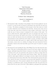
Portfolio Selection 103<br />
• The efficient frontier, with all weights constrained to<br />
be non-negative, was found by quadratic<br />
programming <strong>and</strong> is shown in the Figure.
Portfolio Selection 104<br />
• There are three reference portfolios. Michaud states<br />
that<br />
– The index portfolio is roughly consistent with a<br />
capitalization weighted portfolio relative to a world<br />
equity benchmark for the six equity markets.<br />
– The current portfolio represent a typical U.S.-based<br />
investor’s global portfolio asset allocation.<br />
– An equal weighted portfolio is useful as a reference<br />
point.
Portfolio Selection 105<br />
Efficient frontier for the global asset allocation problem.
Portfolio Selection 106<br />
Quadratic programming<br />
• Quadratic programming minimizes over x<br />
subject to<br />
<strong>and</strong><br />
1<br />
2 xT Hx + f T x (16)<br />
Ax ≤ b, (17)<br />
A eq x = b eq . (18)<br />
• N is the dimension of the problem (number of<br />
variables)<br />
• x <strong>and</strong> f are N × 1 vectors <strong>and</strong> H is an N × N matrix.
Portfolio Selection 107<br />
• Also,<br />
– A is m × N <strong>and</strong> b is m × 1 for some m<br />
– A eq is n × N <strong>and</strong> b eq is n × 1 for some n<br />
• In other words, quadratic programming minimizes the<br />
quadratic objective function (16) subject to<br />
– m linear inequality constraints (17) <strong>and</strong><br />
– n linear equality constraints (18).
Portfolio Selection 108<br />
• We can impose nonnegativity constraints on the<br />
weights of a portfolio by solving the minimization<br />
problem above with<br />
* x = ω, H = Ω, f equal to a N × 1 vector of zeros,<br />
* A = −I (the N × N identity matrix), b equal to a<br />
N × 1 vector of zeros,<br />
( ) 1<br />
T<br />
A eq =<br />
µ T ,<br />
* <strong>and</strong><br />
b eq =<br />
( 1<br />
µ P<br />
)<br />
.
Portfolio Selection 109<br />
• Then (16) becomes one-half the variance of the<br />
portfolio’s <strong>return</strong><br />
ω T Ωω/2,<br />
that is, one-half the objective function (1), (17)<br />
becomes the nonnegative constraints ω ≥ 0, <strong>and</strong> (18)<br />
becomes<br />
( 1<br />
T<br />
µ T )<br />
ω =<br />
( 1<br />
µ P<br />
)<br />
.<br />
which is the same as constraints (2) <strong>and</strong> (3).<br />
• Thus, we are solving the same minimization problem<br />
as in “efficient set math” but with the constraint that<br />
all of the ω i be non-negative.
Portfolio Selection 110<br />
• The minimization problem solved by efficient set<br />
math can also be solved by quadratic programming<br />
– just remove the non-negativity constraint<br />
• This is done by redefining<br />
– A to be a vector of zeros <strong>and</strong><br />
– b to be 0.<br />
• With these choices of A <strong>and</strong> b, constraint (17) is that<br />
0 ω i ≤ 0 for all i, which obviously is always satisfied<br />
<strong>and</strong> so has no effect.<br />
• the reason we use a constraint that has no effect is<br />
the MATLAB’s QUADPROG is written so that some<br />
constraint must be input.
Portfolio Selection 111<br />
Here is the documentation for MATLAB’s “quadprog”<br />
illustrating several ways that this program can be used.<br />
• In our applications, e.g., in the program<br />
“portfolio02QP.m,” we call the program “quadprog”<br />
with a comm<strong>and</strong> of the type<br />
“X=QUADPROG(H,f,A,b,Aeq,beq,LB,UB)”.
Portfolio Selection 112<br />
QUADPROG Quadratic programming. X=QUADPROG(H,f,A,b) solves<br />
the quadratic programming problem:<br />
min 0.5*x’*H*x + f’*x subject to: A*x
Portfolio Selection 113<br />
Here is a program to find efficient frontier, minimum<br />
variance portfolio, <strong>and</strong> tangency portfolio with the<br />
constraint of no short selling. First input the data.<br />
bmu = [.08;.03;.05] ;<br />
bOmega = [ .3 .02 .01 ;<br />
.02 .15 .03 ;<br />
.01 .03 .18 ] ;<br />
Then A eq is defined.<br />
Aeq = [ones(1,length(bmu));bmu’] ;<br />
Then we create a grid of 50 µ P values from .03 to .08.<br />
ngrid = 50 ;<br />
muP = linspace(.03,.08,ngrid) ;
Portfolio Selection 114<br />
Then we set up matrices for storage<br />
sigmaP = muP ; % Set up storage<br />
sigmaP2 = sigmaP ;<br />
omegaP = zeros(3,ngrid) ;<br />
omegaP2 = omegaP ;<br />
rf = .04 % This is the <strong>risk</strong>-free rate<br />
Finally, we find the portfolio weights for each value of µ P .<br />
for i = 1:ngrid ;<br />
omegaP(:,i)=quadprog(bOmega,zeros(length(bmu),1),’’,’’, ...<br />
Aeq,[1;muP(i)],zeros(3,1)) ;<br />
end ;
Portfolio Selection 115<br />
We can also find the minimum variance portfolio <strong>and</strong> the<br />
tangency portfolio.<br />
imin=find(sigmaP==min(sigmaP)) ;<br />
ieff = (muP >= muP(imin)) ;<br />
sharperatio = (muP-rf) ./ sigmaP ;<br />
itangency = find(sharperatio == max(sharperatio)) ;<br />
plot(sigmaP(ieff),muP(ieff),sigmaP(itangency),muP(itangency), ...<br />
’*’,sigmaP(imin),muP(imin),’o’,0,rf,’x’) ;<br />
line([0 sigmaP(itangency)],[rf,muP(itangency)])
Portfolio Selection 116<br />
0.08<br />
0.075<br />
0.07<br />
<strong>expected</strong> <strong>return</strong><br />
0.065<br />
0.06<br />
0.055<br />
0.05<br />
0.045<br />
0.04<br />
0 0.1 0.2 0.3 0.4 0.5 0.6<br />
st<strong>and</strong>ard deviation of <strong>return</strong>