Problem P6-9a, b, c, Fogler The elementary liquid-phase series ...

Problem P6-9a, b, c, Fogler
The elementary liquid-phase series reaction
k 1 k 2
A ---------> B ---------> C
is carried out in a 500 dm 3 batch reactor. The initial concentration of A is 1.6 mol/dm 3 . The desired
product is B and separation of the undesired product C is very difficult and costly. Because the
reaction is carried out at a relatively high temperature, the reaction is easily quenched.
Additional information:
Cost of pure reactant A = $10/mol A
Selling price of pure B = $50/mol B
Separation cost of A from B = $50/mol A
Separation cost of C from B = $30 (e 0.5Cc - 1)
k1 = 0.4 h -1
k2 = 0.01 h -1 at 100 o C
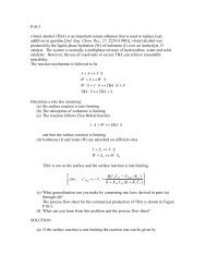
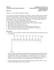
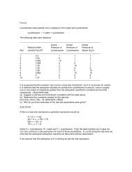
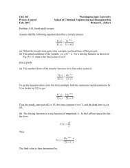
(a) Assuming that each reaction is irreversible, plot the concentrations of A, B, and C as a function
of time.
(b) Calculate the time the reaction should be quenched to achieve the maximum profit.
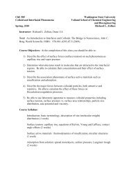
(c) For a CSTR space-time of 0.5 h, what temperature would you recommend to maximize B? (E 1 =
10,000 cal/mol, E 2 = 20,000 cal/mol).
SOLUTION
For parts a), and b) of this problem we are dealing with a constant volume batch rector in which a
liquid phase reaction occurs. We can assume, therefore, that the volume remains constant.
Dividing the material balances for A, B and C by the volume gives the three material balances
dC A /dt = -k 1 C A
dC B /dt = k 1 C A - k 2 C B
dC C /dt = k 2 C B
Note we could also replace the last material balance by an overall balance
C C = C Ao + C Bo + C Co - C A - C B
but let's solve this using the three ODE's. First define the constants in the problem.
k 1 := 0.4
k 2 := 0.01
C Ao := 1.6
C Bo := 0

C Co := 0
V := 500
y :=
⎛
⎜
⎜
⎜
⎝
C Ao
C Bo
C Co
⎞
⎟
⎟
⎟
⎠
D( t,
y)
:=
⎛
⎜
⎜
⎜
⎝
−k 1 ⋅y 0
k 1 ⋅y 0 − k 2 ⋅y 1
k 2 ⋅y 1
⎞
⎟
⎟
⎟
⎠
Z := Rkadapt( y, 0, 200, 200,
D)
ii := 0..
200
2
Concentration Profile
1.5
Concentration (mol/dm^3)
1
0.5
0
0 50 100 150 200
Time (hours)
CA
CB
CC

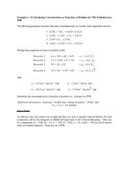
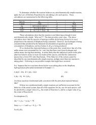
) For part (b) we need to compute the profit that would be generated. Since we have all of the
concentrations as a function of time we can use this information to compute the profit. The profit
would be given by
P = - C Ao
*V*$10 + C B
*V*$50 + C A
*V*$10 - C A
*V*$50 - $30*(e 0.5*CC - 1)
where the first, fourth and fifth terms are negatives because these are costs of the operation. The
second term is positive as this represents the creation of the product B. The third term represents a
credit to process from the recovery of unused A. The profit is thus given by
Z ( ii,
4)
:= −10
⋅
C Ao
⋅⎡⎣ ⎡⎣ ( ) ⎤⎦ − 1⎤⎦
⋅V
+ 50⋅Z ( ii,
2)
⋅V
+ 10⋅Z ( ii,
1)
⋅V
− 50⋅Z ( ii,
1)
⋅V
− 30 exp 0.5⋅Z ii,
3
Now plot the profit as shown below
4 . 10 4 Profit from Batch Process
2 . 10 4
Profit ($)
2 . 10 4 0
4 . 10 4
0 50 100 150 200
Reaction Time (hours)
To the nearest hour the maximum in the profit occurs at t = 11 hours with a profit of $27,850.
Part c) We now need to solve this problem for a CSTR and determine an optimum temperature.
The first thing to do is to express the two rate constants as functions of temperature. First compute
the preexponential factor.
k 1
A 1 :=
−10000
exp⎛
⎜
1.987⋅373
⎝
k 2
A 2 :=
−20000
exp⎛
⎜
1.987⋅373
⎝
⎞
⎟
⎠
⎞
⎟
⎠
A 1 = 2.896 × 10 5
A 2 = 5.242 × 10 9

The material balance for A in a CSTR is given by
0 = F Ain - F Aout + r A V = vC Ain - vC Aout - k 1 C Aout V
but since we are assuming constant volumes (liquid phase reaction) this can be rearranged to give
or
0 = C Ain
- C Aout
- k 1
C Aout τ
C Aout
= C Ain
/(1 + k 1 τ)
Similarly the material balance for B gives
0 = C Bin
- C Bout
+ k 1
C Aout τ − k 2
C Bout τ
Since C Bin = 0 and we have already solved the material balance to get C Aout the material balance for
B can be expressed as
0 = -C Bout
+ k 1 τC Ain
/(1 + k 1 τ) - k 2
C Bout τ
Solve this equation for C Bout to get
k 1 τC Ain
/(1 + k 1 τ)
C Bout
= _______________
(1 + k 2 τ)
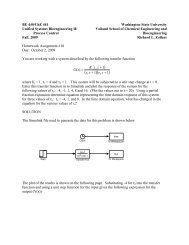
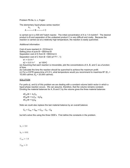
Our problem now is to find where C Bout is a maximum as a function of temperature. We could do
this by plotting the expression above as a function of temperature and visually seeing where the
maximum occurs.
τ := 0.5
T ii := 300 + ii
k 1 ( T) := A 1 ⋅exp
k 2 ( T) := A 2 ⋅exp
C Bout ( T)
:=
⎛
⎜
⎝
⎛
⎜
⎝
−10000
1.987⋅T
−20000
1.987⋅T
k 1 ( T) ⋅τ⋅C Ao
( 1+
k 1 ( T) ⋅τ)
1 + k 2 ( T) ⋅τ
⎞
⎟
⎠
⎞
⎟
⎠

0.8
CB Dependence on Reactor Temperature
0.6
CB (mol/dm^3)
0.4
0.2
0
300 350 400 450 500
Temperature (K)
Thus the maximum in C Bout occurs at a temperature between 436 and 437 K. The maximum value
for C Bout is 0.75 mol/dm 3 . Another way to approach this problem is to find the maximum in C Bout by
differentiating the expression for C Bout with respect to T and setting the differential to zero. The
differentiation and root finding for this problem is going to require quite a bit of algebra. Since this
would also introduce a high probability of error let's use the abilities of MathCAD to do this for us.
The first thing we want to do is to use the symbolic manipulator to perform the differentiation. To
keep the expression for the derivative relatively shorter we do not want it to calculate numerical
values (since it will display these as numbers with 16 decimal figures). So use a symbol to
represent E/R for each rate constant.
E1R :=
E2R :=
−10000
1.987
−20000
1.987
Now write just the right hand side of the expression for C Bout (or highlight just the right had side of
the expression above , copy it and past the copy below
⎛
A 1 exp⎜
E1R ⎞
⋅ ⎟⋅τ⋅C Ao
⎝ T ⎠
⎛
⎜1+
A 1 ⋅exp⎛
⎜
E1R ⎞
⎟⋅τ⎞
⎟
⎝ ⎝ T ⎠ ⎠
1 + A 2 ⋅exp⎛
⎜
E2R ⎞
⎟⋅τ
T
⎝
⎠

To perform the differentiation first place the cursor on one of the "T's" in the expression above.
Then go to the menu bar at the top of the screen and click on "Symbolics". In the menu that
appears click on "Variable" and on the subsequent menu click on "Differentiate". The derivative
of the expression with respect to T will appear below. As the expression below appeared
originally it spread over three pages. I have edited this expression by inserting a line break just
before some of the "+" signs. To do this I put the cursor just before the "+" sign, hit the space
bar until the entire previous term was selected then pressed CTRL+ENTER.
⎡
⎢
⎢
⎣
⎛
⎝
⎞
⎟
⎠
C Ao
⎤
⎞⋅ ⎛ ⎥
⎛ ⎞
⎜⎝ ⎟⋅τ⎞ ⎤ ⎟⎠ ⎥ ⎥
⎠ ⎦ ⎦
E1R
−A 1 ⋅ ⋅exp⎜
E1R ⋅τ⋅
T 2 T ⎛1 A 1 exp⎛
⎜
E1R ⎞
⎜ + ⋅
⎝ T ⎟⎠ ⋅τ⎟
⎝
⎠ 1 A 2 exp⎜
E2R
...
⎡
⎢
+ ⋅
⎣
⎝ T
⎡
2
2 E1R
A 1 ⋅ exp
⎛ ⎞
⎜ ⎟ τ 2
C ⎢⎢⎢⎣
Ao
E1R⎤ +
⋅ ⋅
⋅ ⎥⎥⎥⎦ ...
⎝ T ⎠ ⎡ ⎛ 1 + A 1 ⋅exp⎛
⎜
E1R ⎞
⎜⎝ ⎟⋅τ
⎞ 2
⎢⎣
⎟⎠ ⋅⎛1 + A 2 ⋅exp⎛
⎜
E2R ⎞
⎜
⎝ T ⎠
⎝ T ⎟⎠ ⋅τ⎞
⎤ T 2
⎟ ⎥⎦
⎝
⎠
A 1 ⋅ exp⎛
⎜
E1R ⎞
⎟⋅
⎝ T ⎠
τ 2
C Ao
E2R
+
⋅ ⋅A 2 ⋅ ⋅exp⎛
⎜
E2R
⎡
⎢⎛1 + A 1 ⋅exp⎛
⎜
E1R ⎞
⎜
⎝ T ⎟⎠ ⋅τ⎞
⎟
⎛ ⎝
⎠ 1 + A 2⋅exp⎛
⎜
E2R ⎞
⎜⎝ ⎟⋅τ
⎞ 2 ⎤ T
⋅
⎟⎠ ⎥
2 ⎝ T
⎣
⎝ T ⎠ ⎦
⎞
⎟
⎠
With this derivative we are now ready to use the root finder in MathCAD. Start by giving an initial
estimate - Note that we must use T as the variable since T appears in the expression of the
derivative. Then type "Given" to start the root finder.
T := 400
Given
We now need to take a copy of the derivative that was determined above, place it below the "Given"
command and then set it equal to zero using the Boolean equal sign.
⎡
⎢
⎢
⎣
⎛
⎝
⎞
⎟
⎠
C Ao
⎤
⎞⋅ ⎛ ⎥
⎛ ⎞
⎜⎝ ⎟⋅τ⎞ ⎤ ⎟⎠ ⎥ ⎥
⎠ ⎦ ⎦
E1R
−A 1 ⋅ ⋅exp⎜
E1R ⋅τ⋅
T 2 T ⎛1 A 1 exp⎛
⎜
E1R ⎞
⎜ + ⋅ ⎟⎠ ⋅τ⎟
⎝ ⎝ T ⎠ 1 A 2 exp⎜
E2R
...
⎡
⎢
+ ⋅
⎣
⎝ T
⎡
2
2 E1R
A 1 ⋅ exp
⎛ ⎞
⎜ ⎟ τ 2
C ⎢⎢⎢⎣
Ao
E1R⎤ +
⋅ ⋅
⋅ ⎥⎥⎥⎦ ...
⎝ T ⎠ ⎡ ⎛ 1 + A 1 ⋅exp⎛
⎜
E1R ⎞
⎜⎝ ⎟⋅τ
⎞ 2
⎢⎣
⎟⎠ ⋅⎛1 + A 2 ⋅exp⎛
⎜
E2R ⎞
⎜
⎝ T ⎠
⎝ T ⎟⎠ ⋅τ⎞
⎤ T 2
⎟ ⎥⎦
⎝
⎠
A 1 ⋅ exp⎛
⎜
E1R ⎞
⎟⋅
⎝ T ⎠
τ 2
C Ao
E2R
+
⋅ ⋅A 2 ⋅ ⋅exp⎛
⎡
⎢⎛1 + A 1 ⋅exp⎛
⎜
E1R ⎞
⎜
⎝ T ⎟⎠ ⋅τ⎞
⎟
⎛ ⎝
⎠ 1 + A 2⋅exp⎛
⎜
E2R ⎞
⎜⎝ ⎟⋅τ
⎞ ⎜
E2R
2 ⎤ T
⋅
⎟⎠ ⎥
2 ⎝ T
⎣
⎝ T ⎠ ⎦
Now find the root by using the "find" command.
⎞
⎟
⎠
= 0

T opt
:=
Find( T)
T opt = 436.848
C Bout ( T opt ) = 0.75

aterial balance for