COMSOL Multiphysics (formerly FEMLAB) is a finite element ...

COMSOL (FEMLAB) TUTORIAL
COMSOL Multiphysics (formerly FEMLAB) is a finite element analysis and solver software
package for various physics and engineering applications, especially coupled phenomena, or
multiphysics. COMSOL Multiphysics also offers an extensive and well-managed interface to
MATLAB and its toolboxes for a large variety of programming, preprocessing and
postprocessing possibilities. In addition to conventional physics-based user-interfaces,
COMSOL Multiphysics also allows for entering coupled systems of partial differential
equations (PDEs).
How to create a new model in Comsol
1. Start Comsol Multiphysics and create a new file (menu File) indicating the PDE’s to be
used.
2. Define the geometry (menu Draw)
3. Enter the variables needed and boundary conditions in each equation for every
subdomain (menu Physics)
4. Choose the element size to be used in the calculations (menu Mesh)
5. Choose the type of numerical solver (menu Solve)
6. Display the results in the most convenient way (menu Postprocessing)
7. The menu Multiphysics is to perform changes in the model by adding or removing
equations.
Not all of these steps are always necessary when building a model. The order is also variable
depending on the complexity of the model.
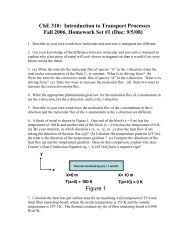
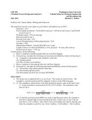
Example 1 (HEAT TRANSFER)
Consider a cylindrical heating rod which is sheathed by a concentric tube of thickness 0.05 m.
The entire assembly is immersed in a fluid and the system is at steady-state, as shown below.
We wish to determine the temperature distribution within the sheath. After thinking about the
problem, assume that we arrived at the following approximations (make sure you understand
how we arrived to following approximations for your future quiz and test):

The temperature of the heater is constant at 400K.
The temperature at R1 is the same as the temperature of the heater, 400K.
The fluid temperature is constant at 300K and this is the temperature of the surrounding sheath
at R2.
Given the symmetry of the system, it will enough for the analysis to define a subdomain in 2D
as shown below.
Solution using Comsol Graphical User Interface.
1. To start Comsol, click the icon COMSOL Multiphysics 3.2
2. In the Model Navigator window we
must choose the type of coordinate
system that we want to use to solve our
problem. As mentioned above, our
problem is pretty symmetric and
therefore a 2D system (which is the
default value) will be enough.

3. Next, we need to provide
information about the application
modes (or PDE’s) that must be
taken into consideration in order to
solve our problem. In accordance
with the statement, the problem
can be solved considering only
conductive heat transfer. Hence,
we must select this application
mode and to do so, we must
double-click the option COMSOL
multiphysics.
4. Next, we double click on the option Heat Transfer.
5. Next, select the option Conduction by doing one click on the symbol “+” to the left. In
doing so two new options will show up. We must pick one of them depending on the type
of regime we will use to solve our problem. For our case we select Steady-state analysis
doing one click on this option.

8. Once we select the regime three new fields will be activated at the bottom of the window.
The field Dependant variables is to specify a name for the dependant variable. Let us keep
the default name T for the variable temperature.

9. Likewise, let us change the name of the application mode (PDE) from ht (default name) to
Conduction.
8. The third field has to do with the numerical calculations. Let us keep the same value for the
time being. Once we have done this we click on OK. A new window will pop up as shown
below.

9. Before going any further, let us save our work. To do so, we click on the menu File and
then on the option Save As.
To save our work we must specify the path and the name of the file. Let us call our model
Heat transfer. After doing this, we must click on the button Save. The file will be saved
with the extension “mph”.

10. The next step is to specify the geometry of our system. The idea is to use as few figures as
possible to define our system. For our case, the symmetry of the system allows us to use
one single rectangle to define our model. Thus, to draw a rectangle we click on the menu
Draw, then on the option Specify objects and finally on the option Rectangle.
In the new window showing up we specify the size and the position of the rectangle we are
drawing. Since we have to specify dimensions we must be careful with the values we will
enter. The International System of Units (SI) is the default option. Thus, the dimensions of
our rectangle will be 0.3 m and 0.05 m for width and height, respectively. The position is
not important for this case and therefore we will keep the default values. After entering the
values we click on OK.

The rectangle just drawn will be displayed as shown below
To zoom in the rectangle we must click the button at the center and the top of the
screen. After that, we press the left button of the mouse and drag the mouse to cover the
object. Finally, we release the left button of the mouse and the object will look bigger as
shown below.

11. Next, we must click on the menu Physics and then on the option Subdomain Settings to
define the parameters needed by the PDE to be solved. We can also do this by pressing the
key F8. The following window will show up.
Every region in our drawing is called a subdomain. Since we only have one rectangle then
the area of this object will be the subdomain 1. Next, we have to specify the material the
concentric tube is made of in order to use their properties in the calculations. To do so, we
select the subdomain 1, click the field Load… and select Copper from the Library of
materials. Then we click OK.

The properties of copper will be loaded on the subdomain 1 as shown below.
12. After clicking OK we are ready to specify the boundary conditions needed to solve the
PDE. To achieve this, we must click on the menu Physics and the option Boundary
Settings or simply press the key F7. The following windows will be displayed.
In the subdomain 1 we have 4 boundaries and we must specify each of them in order to
solve the model. The boundary currently specified will show up selected with a red arrow
as shown below. For the boundary 1 the temperature is known and equal to 300 K. To

indicate this we select the option Temperature in the field Boundary condition and enter
the value in the field T 0 . Finally, we click Apply and define the next boundary.
For the boundary 2 the temperature is that of the rod (400 K).

For the boundary 3, the temperature is 300 K.
Finally, the temperature in the boundary 4 is 300 K.

13. After clicking OK, we are now ready to run the model. To do so, we must click on the icon
on the top of the screen and the model will be solved. The results are displayed as
shown below.
To view the temperature in each point we must click on any point inside the subdomain and
the value will be displayed at the bottom of the screen.
Postprocessing
The menu Postprocessing will
facilitate us to analyze the information
in different ways. Thus, if we want to
display the variation of the temperature
in a 3D plot instead of a 2D one we
can click the menu Postprocessing
and then the option Plot parameters
(or just simply pressing the key F12).
The following window will be shown.

Next, we select the tag Surface (if not
selected) and click on the button Height
data. After this, we must make sure that
the box Height data is also checked to
be able to activate the fields that define
the variable to plot.
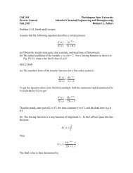
Next, we click OK and the 3D plot
will be displayed as follows. (The
3D plot can be turned by pressing
the left button of the mouse and
dragging it at any direction we
want)
Radius
Temperature
Length

Another possibility is to obtain a temperature profile at certain cross section. This can be
achieved by using the option Cross Section Plot Parameters in the same menu
Postprocessing.
In the window showing up we must specify two points that define the cross section (if working
on 2D). For instance, if we want a temperature profile along the section defined by the points
(0.2,0) and (0.2,0.05) we enter these values in the box entitled Cross-section line data as
shown below.

After clicking OK the section will be marked on the graph as a red line and the following
graph with the temperature profile will be displayed.
Some changes in the
model can be easily
performed. Thus, to
observe how the
temperature changes as
we change the boundary
conditions let us do as
follows. If the boundaries
1 and 4 were very short
then the amount of heat
going out from them can
be assumed to be negligible and therefore those boundaries can be considered as insulated. To
perform these changes in the boundaries we press the key F7 and select the boundaries 1 and 4
at once using the Control key. Then, we change the boundary condition to Thermal
insulation instead of Temperature as shown above.

After clicking OK and running the model, the following result must be obtained.
If the fluid used in the system is not contained in the library we can specify its properties
manually by pressing the key F8 to open the Subdomain settings window. For example, let us
assume that the thermal conductivity were 0.1T 3 +50T 2 -10T+5 W/m.K and the density and the
heat capacity, 1100 Kg/m 3 and 100 J/Kg.K respectively. This data is entered as shown below.
After clicking OK and running the model we obtain the following temperature profile at the
cross section defined above.