design and control of a robot with one articulated leg for locomotion ...

DESIGN AND CONTROL OF A ROBOT WITH ONE
ARTICULATED LEG FOR LOCOMOTION ON IRREGULAR
TERRAIN
H. De Man, D. Lefeber & J. Vermeulen
Vrije Universiteit Brussel, Department of Mechanical Engineering, Pleinlaan 2, 1050 Brussels, Belgium
Hans De Man: tel: +32-2-629.28.08, fax: +32-2-629.28.65, e-mail: hdman@vub.ac.be
Internet: http://wwwtw.vub.ac.be/ond/werk/multibody.htm
1. Introduction
The design of an electrically actuated robot with one articulated leg is presented, as well as simulation
results of its control algorithm. The algorithm enables the robot, whose name is OLIE (One Leg Is
Enough), to control simultaneously its forward velocity during flight, its hopping height, the placement
of its foot on desired footholds, the orientation of its body and its angular momentum, making
locomotion on irregular terrain possible.
The model of the hopping robot under study is given in section 2. The design of the experimental
prototype is presented in section 3, whereas the control algorithm is described in section 4.
Simulation results are presented in section 5 and conclusions are drawn in section 6.
2. A hopping robot with one articulated leg
The control of a running machine is more critical than the control of a walking machine. To be able to
study all the features of a running machine, such as its underactuated and nonholonomic nature,
without unnecessarily increasing the complexity of its design, a robot having one articulated leg is

considered here. For the same reason its motion is restricted to the sagittal plane, which leads to 5
DOF during flight and 3 DOF during stance.
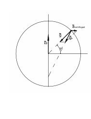
Figure 1 depicts the robot at the moment of take-off (to), and at the moment of touch-down (td).
The robot consists of three segments: a lower leg, an upper leg and a body, connected to each other
by actuated rotational joints. Point F is the foot of the robot, point K its knee and point H its hip. The
center of mass of the body coincides with the hip.
Fig. 1: robot at take-off and at touch-down
3. Mechanical layout and control scheme
OLIE (One Leg Is Enough) is the electrically actuated prototype of the robot described above, its
mechanical layout being given in figure 2a. Of each link the length l, the mass m and the moment of
inertia I com around the center of mass are given in table 1:
Table 1: prototype parameters
l (m) m (kg) I com (kgm 2 )
body 0.666 8.507 0.7979
upper leg 0.308 1.373 0.0218
lower leg 0.342 1.781 0.0138
The robot’s motion is restricted to the 2D surface of a cylinder by a boom mechanism connected to
the robot at its hip, as is shown in figure 2b. The boom is made of a lightweight composite tube and
has a length variable between 2 m and 3 m.

Fig. 2a: Mechanical layout
Fig. 2b: OLIE and its boom mechanism
The upper and lower leg of the robot are built up by aluminium and wooden parts in order to get a
lightweight construction. The upper body is an aluminium frame, horizontally placed upon the leg. A
rubber cushion located at the bottom of the lower leg is referred to as the foot.
Two SEM HD55G4-44S AC brushless servomotors actuating hip and knee respectively are located
at the ends of the upper body, thus assuring a high ratio of body inertia to leg inertia such that during
flight body pitching is minimised. The motors are steered by IRT BR1306 AC-servo-controllers.
To transfer the torques produced by the motors to the corresponding joint, and to transform the high
speed-low torque characteristics of the motors to the low speeds and high torques necessary to
drive the robot, two Synchroflex T5 toothed belt transmission loops were introduced. Each belt loop
is formed by two sub-loops resulting in a total gear ratio of 1:20 for both the hip and the knee.
Combined with this gear ratio, the actuators generate a peak stall torque of 58 Nm at both the hip
and the knee. Maximum power supply is approximately 1.2 kW, one motor weighing only 1.9 kg.
Two carbon steel torsional springs, forming the passive part of the robot’s actuation, are placed at
the knee, exerting a torque as a function of the relative angle between upper and lower leg. Each of
the springs has a spring constant of 45 Nm/rad and a mass of 0.186 kg.
In order to provide measurements of the absolute position of the robot, two sensors are mounted on
the boom pivot. A multi-turn potentiometer is used to determine the horizontal position of the robot’s
hip, while a single-turn potentiometer measuring the angle between boom and pivot, is used to
determine the vertical position of the hip. Three more sensors mounted on the robot yield the
orientation of the different links.

A mechanical switch located at the foot senses contact with the ground.
All calculations concerning the robot’s control are performed in LABVIEW on a Pentium-S PC. The
link between the PC and the servocontroller on one hand and between the sensors on the robot and
the PC on the other hand is formed by a National Instruments AT-MIO-16E-10 data acquisition
board.
A schematic representation of the control system for one actuator, which is based on the principle of
cascade control [1] , is given in figure 3.
Fig. 3: Cascade control structure of a joint of the robot
The angle θ R is the actual relative angle in a joint of the robot measured by a potentiometer and S is a
Boolean variable representing the state of the contact-switch on the foot. Whenever a transition from
flight to stance phase or vice versa occurs, the value of S changes and the control algorithm
*
described in the next paragraph calculates a nominal trajectory θ . This nominal trajectory has to be
R
tracked during this phase in order to attain the desired values of the objective parameters. The BR
1306 servocontroller, which expects a DC voltage V between -10V and +10V as an input, PI-
A
controls the shaft speed
*
n so that only the trajectory for the angular velocity θ & of the link of the
A
robot is tracked. An uncontrolled error between the desired trajectory of the angle
actual trajectory
θ R
θ * and the
R
can occur. Therefore, the control system is extended by a position control loop
R

*
superimposed on the existing speed loop, being a PI-controller acting on the signals θ R
and θ .
R
*
Hence, a correction term ∆ θ & *
R
is added to the trajectory of θ & in order to remove deviations from
*
the desired trajectory of the angle θ .
R
R
4. The control algorithm
To allow the motion of a legged machine to be flexible in terms of locomotion criteria or goals to be
reached, as opposed to steady-state behaviour, it is necessary to take as control variables those
parameters that are linked to the desired behaviour as closely as possible, which leads to the concept
of objective locomotion parameters [2] . When moving on irregular terrain for example, it makes more
sense to express the locomotion pattern in terms of the coordinates of the feet than in terms of the
internal angles between the different links of the machine. The control algorithm presented here is
based on this objective parameters approach, thus broadening locomotion limits such as encountered
in [3] .
The core of the first part of the control algorithm is similar to the algorithm presented in [4] . It focuses
on the flight phase and is formed by the relationships between the equations dictating the parabolic
trajectory of G during flight, and a subset of the parameters to be controlled, being the forward
velocity of G, the jumping height and the position of the foot at touch-down. Using these
relationships, the angles θ 1 and θ 2 needed at take-off and at touch-down, as well as their
corresponding angular velocities and angular accelerations, are calculated. Next, trajectories for θ 1
and θ 2
are generated, for both the flight phase and the stance phase, satisfying the conditions at takeoff
and touch-down. The motor actuating the knee then tracks the trajectory for θ 1 , the motor
actuating the hip tracks the trajectory for θ 2 .
Since the angle θ 3
between the body and the horizontal does not appear in the expressions giving the
trajectory of G, the first part of the control algorithm is not able to control the body’s orientation. To
prevent destabilization of the locomotion due to rotation of the robot’s body, a second part in the
control strategy is needed. Therefore the nonholonomic constraints expressing that the angular
momentum around G during flight is constant and that the angular momentum around the foot during
stance only depends on gravity, have to be taken into account. By integrating these constraints and
by expressing that the angle θ 3
and the angular momentum around G have to be equal to preset
values at take-off, correction functions for the trajectories of θ 1
and θ 2
during stance are calculated.
These functions are chosen in such a way that they respect the values for θ 1 and θ 2 , as well as the

values of their first and second derivatives, at take-off and at touch-down. In this way, by adding the
correction functions to the initial trajectories and by letting the actuators track the new trajectories,
the orientation of the body of the robot is controlled, without altering the robot’s forward velocity, its
hopping height or the placement of its foot. The desired values of all these objective locomotion
parameters can be altered from one hop to another.
5. Simulation results
Figures 4 to 9 show some simulation results for two consecutive hops, with the values of the
*
*
*
desired objectives (the step length D x F
, the stepping height D y F
, the forward velocity x&
G
, the
*
to,*
hopping height D h , the orientation of the body at take-off θ
to ,*
G at take-off µ ) being identical for each hop and given by:
G
*
D x F = 0.2 m;
*
D y F = 0.0 m;
*
x&
G = 0.5 m/s;
D h * = 0.05 m;
3
and the angular momentum around
to,*
θ
3 = 0. 0 rad;
to,*
µ
G = 0.0 kgm 2 /s
x F (m)
0.4
dx G /dt(m/s)
0.5
0.2
flight stance flight stance
0.0
0.0 0.2 0.4 0.6 0.8
t(s)
flight stance flight stance
0.0
0.0 0.2 0.4 0.6 0.8
t(s)
Fig. 4: horizontal position of the foot vs. time
y G(m)
0.5
θ 3(rad)
0.1
0.0
Fig. 5: forward velocity vs. time
controlled
flight stance flight stance
0.0
0.0 0.2 0.4 0.6 0.8
t(s)
uncontrolled
-0.1
flight stance flight stance
-0.2
0.0 0.2 0.4 0.6 0.8 t(s)
Fig. 6: vertical position of G vs. time
Fig. 7: orientation of the body vs. time

µ G(kgm 2 /s)
T(Nm)
0.4
50
0.0
controlled
knee
hip
uncontrolled
0
-0.4
flight stance flight stance
-0.8
0.0 0.2 0.4 0.6 0.8
t(s)
flight stance flight stance
-50
0.0 0.2 0.4 0.6 0.8 t(s)
Fig. 8: angular momentum around G vs. time
Fig. 9: actuator torques vs. time
Figure 4 shows the horizontal position x F
of the foot versus time. The step length is given by the
distance between the two successive horizontal parts in the graph and is equal to the desired value.
Figure 5 shows the forward velocity x& of the global center of mass versus time. The velocity during
G
the flight phases equals the desired value. The vertical position y G
of the global center of mass of the
robot is given in figure 6. The horizontal line at the bottom indicates the height of G at take-off,
whereas the other horizontal line indicates the maximum height. The distance between the two lines
gives the hopping height, being equal to the desired value. Figures 7 and 8 represent respectively the
orientation of the body θ 3 and the angular momentum around G versus time. Without the second part
of the control strategy the drift in the body’s orientation as well as in the robot’s angular momentum
is clearly visible. Adding the extra control positions the body horizontally at take-off and makes the
angular momentum at take-off equal to its desired zero value.
The actuator torques needed to sustain the robot’s motion stay below the limits of 58 Nm of the
motors used for the prototype, as can be seen on figure 9.
To test the robot’s ability to vary the objective locomotion parameters during hopping, simulations
with two different consecutive hops have been done, using the following values:
*
hop 1: D x F
= 0.25 m;
*
hop 2: D x F = 0.33 m;
*
x&
G = 0.65 m/s
*
x&
G = 0.70 m/s
The results visualized by figures 10 and 11 show that the robot behaves in the desired way. From the
first hop to the second one the step length and the forward velocity change as they should, with the
control on the orientation of the body and the robot’s angular momentum also working correctly.

x F (m)
dx G /dt(m/s)
0.5
0.7
flight stance flight
0.0
0.0 0.2 0.4 0.6
t(s)
flight stance flight
0.0
0.0 0.2 0.4 0.6
t(s)
Fig. 10: horizontal position of the foot vs. time
Fig. 11: forward velocity vs. time
Figures 4 to 11 show that the control strategy presented in this paper works very efficiently, since
controlled periodic hopping, as well as controlled aperiodic hopping can be achieved.
6. Conclusion
An electrically actuated prototype of a robot with one articulated leg has been built and its design is
presented. The outlay is given of a control algorithm enabling the robot to control simultaneously its
forward velocity during flight, its hopping height, its step length, its stepping height, the orientation of
its body and its angular momentum. Simulation results show that the algorithm is efficient and that the
desired objectives are attained. A robot using this algorithm should be able to jump over obstacles
and to move over terrain where footholds are randomly distributed.
On the theoretical level future research will focus on the robustness of the control algorithm and on
the determination of the physically admissible subspace, in terms of actuator and geometrical
constraints, of the space formed by the controlled parameters. On the practical level the control
strategy will be implemented on the mechanical prototype and the experimental results will be
compared to the simulated ones.
References
[1] W. Leonhard, Control of Electrical Drives, 1985, Springer-Verlag, Berlin.
[2] Y. Hurmuzlu , 1993, "Dynamics of Bipedal Gait Part I: Objective Functions and the Contact Event of a Planar
Five-Link Biped", Journal of Applied Mechanics, 60, pp. 331-336.
[3] J.K. Hodgins & M.H. Raibert, 1991, "Adjusting Step Length for Rough Terrain Locomotion", IEEE
Transactions on Robotics and Automation, 7(3), pp. 289-298.
[4] H. De Man, D. Lefeber, F. Daerden & E. Faignet, 1996, "Simulation of a New Control Algorithm for a One-
Legged Hopping Robot (Using the Multibody Code MECHANICA Motion)", in: Proceedings International
Workshop on Advanced Robotics and Intelligent Machines, Manchester, UK.