Suggested Solutions to Assignment 2 - Department of Economics

ECON 2450 

Intermediate Macroeconomic Theory II 

Instructor: Sharif F. Khan 

Department of Economics 

York University 

Winter 2013 

Suggested Solutions to Assignment 2 (OPTIONAL) 

Total Marks: 25 

Read each part of the question very carefully. Show all the steps of your calculations to 

get full marks. 

B1. (5 marks) 

Consider two hypothetical countries: Home and Foreign. Home makes ordinary 

soap bars that are sold for 5 dollars each. Foreign makes deluxe soap bars that are 

sold for 100 yens each. The real exchange rate between Home and Foreign is a half 

of the deluxe soap bar per ordinary soap bar. 

(i) What is the nominal exchange rate between the Home dollar and the 

Foreign yen? 

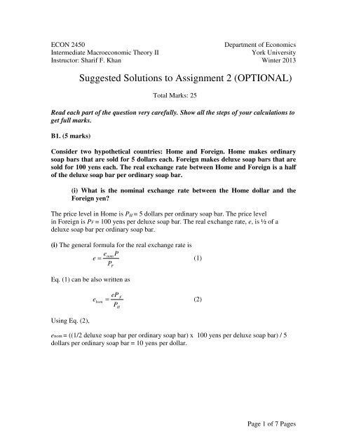
The price level in Home is P H = 5 dollars per ordinary soap bar. The price level 

in Foreign is PF = 100 yens per deluxe soap bar. The real exchange rate, e, is ½ of a 

deluxe soap bar per ordinary soap bar. 

(i) The general formula for the real exchange rate is 

enomP 

e = (1) 

P 

Eq. (1) can be also written as 

Using Eq. (2), 

F 

eP 

F 

e 

bom 

= (2) 

PH 

enom = ((1/2 deluxe soap bar per ordinary soap bar) x 100 yens per deluxe soap bar) / 5 

dollars per ordinary soap bar = 10 yens per dollar. 

Page 1 of 7 Pages

(ii) During the following year, Home has 10% domestic inflation and Foreign 

has 20% domestic inflation. The real exchange rate remains unchanged. At 

the end of the year, what has happened to the nominal exchange rate? Which 

country has had a nominal appreciation? Which has a nominal depreciation? 

Inflation in Home is π H = 10%. Inflation in Foreign is π F = 20%. The real exchange rate is 

constant. 

We can write Eq. (2) in the percentage change form as 

∆e 

e 

nom 

nom 

= 

∆e 

∆P 

+ 

e P 

F 

F 

∆P 

− 

P 

= 

∆e 

+ π 

F 

− π 

e 

H 

(3) 

∆enom 

So, = 0 + 0.20 − 0.10 = 0. 10 . 

e 

nom 

Therefore, the nominal exchange rate (yens per dollar) has increased by 10%. The Home 

dollar has appreciated, the Foreign yen has depreciated. 

B2. (20 marks) 

Consider the following Keynesian small open economy: 

Desired Consumption: C d = 200 + 0.6( Y − T ) − 200r 

Desired Investment: 

I d = 300 − 300r 

Government Purchases: G = 152 

Taxes: 

T = 20 + 0. 2Y 

Net Exports: 

NX = 170 − 0.08Y 

− 0. 5e 

Real exchange rate: e = 230 

Real Money Demand: 

L = 0.5Y 

− 200r 

Money Supply M = 924 

Full-employment output: Y = 1000 

Net Factor Payments: NFP = 0 

In this economy, the real interest rate does not deviate from the foreign interest rate. 

a) Derive the equation for the IS curve as a function of Y and e. 

The equation for the IS curve is derived from the goods market equilibrium condition for 

an open economy, which is 

S 

d 

d 

− I = CA = NX + NFP = NX (because, NFP=0). (1) 


S d = Y+NFP - C d - G = Y+0 – {200 + 0.6[Y – (20 + 0.2Y)] – 200r} –152 

= 0.52Y – 340 +200r 

So, S d = 0.52Y – 340 +200r (2) 

It is given that 

NX = 170 − 0.08Y 

− 0. 5e 

and I d = 300 − 300r 

. 

Substituting the functional forms of S d , 

d 

I , and NX into Eq. (1), 

0.52Y – 340 + 200r – (300 – 300r) = 170 – 0.08Y –0.5e. 

Rearranging terms and simplifying gives the IS curve: 

500r = 810 – 0.5e – 0.6Y 

810 5 6 

or, r = − e − Y 

500 5000 5000 

(4) [IS curve] 

b) Derive the equation for the LM curve as a function of Y, M and P. 

The equation for the LM curve is derived from the assets market equilibrium condition 

for an open economy, which is 

M/P = L (5) 

Substituting the given functional form of L into Eq. (5), 

or, 

or, 

M/P = 0.5Y – 200r 

200r = -M/P +0.5Y 

M 5 

r = − Y 

200 P 

2000 

(6) [LM curve] 

c) What are the general equilibrium (that is, long-run) values of output, the real 

interest rate, real exchange rate, consumption, investment, net exports, and 

the price level? Illustrate the general equilibrium values of output and the 

real interest rate in the IS-LM-FE diagram. 

In the general equilibrium, output equals to its full-employment level, which is 1000. 

The given general equilibrium value of real exchange rate, e = 230. 

With e = 230 and Y = 1000, the IS curve (Eq. (4)) gives 

r = 

810 

500 

− 

5 

5000 

6 

5000 

( 230) − ( 1000) = 0. 19 


So, the general equilibrium value of the real interest rate is 19%. 

With r = 0.19 and Y = 1000, the LM curve (Eq. (6)) gives 

924 

0 .19 = − + 

200P 

924 

⇒ = 2.5 − 0.19 

200P 

924 

⇒ P = = 2 

200* 2.31 

5 

( 1000) 

2000 

So, the general equilibrium value of the price level is 2. 

The general equilibrium value of net exports, 

NX = 170- 0.08*1000-0.5*230= 170 – 80 – 115 = –25. 

The general equilibrium value of consumption, 

C= 200 + 0.6(1000 – 20-0.2*1000) – 200*0.19 = 630 

The general equilibrium value of investment, / = 300 – 300*0.19 = 243 

Figure 4(c) illustrates the general equilibrium values of output and the real interest rate in 

the IS-LM-FE diagram. 

d) Starting from the initial general equilibrium, money supply is increased to 

1024. Assuming flexible exchange rates, what are the effects of this change on 

output, the real interest rate, the real exchange rate, consumption, 

investment, and net exports in the short run? Illustrate the short-run 

equilibrium values of output and the real interest rate in the IS-LM-FE 

diagram. 

Start at the general equilibrium derived in part (c), where the general equilibrium real 

interest rate is 19%. So, by assumption, the foreign interest rate is fixed at 19% and the 

domestic real interest rate does not deviate from this level. That is, r = 0.19 holds at any 

short run or long-run equilibrium. 


In the short run, the price level remains fixed at 2. M has increased to 1024. Substituting 

r = 0.19, M = 1024, and P=2 into the LM curve (Eq. (6)), we get 

1024 5 

0.19 = − + Y 

200* 2 2000 

1 

⇒ 0.19 = −2.56 

+ Y 

400 

1 

⇒ Y = 2.75 

400 

⇒ Y = 1100. 

So, the short-run equilibrium value of the output is 1100 (output has increased in the 

short run). 

Substituting r = 0.19 and Y = 1100, and P=2 into the IS curve (Eq. (4)), we get 

810 5 6 

0.19 = − e − 1100 

500 5000 5000 

⇒ 0.19 = 1.62 − 0.001e 

−1.32 

⇒ 0.001e 

= 0.11 

⇒ e = 110. 

So, the short-run equilibrium value of real exchange rate, e = 110 (the real exchange rate 

has depreciated in the short run). 

The short-run equilibrium value of net exports, 

NX = 170 - 0.08*1100 - 0.5*110 = 27 (net exports have increased in the short run). 

The short-run equilibrium value of consumption, 

C= 200 + 0.6(1100 – 20-0.2*1100) – 200*0.19 = 200 + 0.6(860)-38 = 678 (consumption 

has increased in the short run). 

The short-run equilibrium value of investment, / = 300 – 300*0.19 = 243 (investment has 

remained unchanged in the short run). 

Figure 4(d) illustrates the short-run equilibrium values of output and the real interest rate 

in the IS-LM-FE diagram. 


e) Using the same information as provided in part (d), in the long run what 

would happen to output, the real interest rate, the real exchange rate, 

consumption, investment, net exports, the nominal money supply, the price 

level, and the real money supply? Illustrate the new general equilibrium (that 

is, new long-run) values of output and the real interest rate in the IS-LM-FE 

diagram. 

Since at the short-run equilibrium the economy is operating above the full-employment 

level, there is an upward pressure on the price level. In the long-run, the price level will 

fully adjust and output will return to its full-employment level. So, at the new general 

equilibrium output will be equal to 1000. Substituting r = 0.19, M = 1024, and Y=1000 

into the LM curve (Eq. (6)), we get 

1024 5 

0.19 = − + 

200* P 

5.12 

⇒ 0.19 = − + 2.5 

P 

5.12 

⇒ = 2.31 

P 

⇒ P = 2.2165. 

(1000) 

2000 

So, the new general equilibrium value of the price level is 2.2165 (the price level will 

increase in the long run). 

In the long run the nominal money supply will remain unchanged at its new level, 1024. 

At the initial general equilibrium, the real money supply was 924/2 = 462. At the shortrun 

equilibrium, the real money supply increased to 1024/2 = 512. At the new general 

equilibrium, the real money supply will be 1024 / 2.2165 = 461.9896 ≈ 462. 

This means 

that in the long-run the real money supply will return to its initial level. 

Substituting r = 0.19 and Y = 1000 into the IS curve (Eq. (4)), we get 

810 5 6 

0.19 = − e − 1000 

500 5000 5000 

⇒ 0.19 = 1.62 − 0.001e 

−1.2 

⇒ 0.001e 

= 0.23 

⇒ e = 230. 

The new general equilibrium value of real exchange rate, e = 230 (the real exchange rate 

will remain unchanged in the long run). 

The new general equilibrium value of net exports, 

NX = 170- 0.08*1000-0.5*230= 170 – 80 – 115 = –25 (net exports will remain 

unchanged in the long run). 


The new general equilibrium value of consumption, 

C= 200 + 0.6(1000 – 20-0.2*1000) – 200*0.19 = 630 (consumption will remain 

unchanged in the long run). 

The new general equilibrium value of investment, / = 300 – 300*0.19 = 243 (investment 

will remain unchanged in the long run). 

The results of this part of the question show that the monetary neutrality holds in the 

Keynesian long run. Figure 4(e) illustrates the new general equilibrium values of output 

and the real interest rate in the IS-LM-FE diagram.

Suggested Solutions to Assignment 2 - Department of Economics

Create successful ePaper yourself

Delete template?

Save as template?