Sirgue, L., and Pratt, R. G., 2003. - Queen's University

a)
V (m/s)
3500
3000
2500
2000
1500
b)
V (m/s)
3500
3000
2500
2000
1500
Depth (km)
Depth (km)
Distance (km)
0 1 2 3 4 5 6 7 8 9
0
0.5
1.0
1.5
2.0
0
0.5
1.0
1.5
2.0
Distance (km)
0 1 2 3 4 5 6 7 8 9
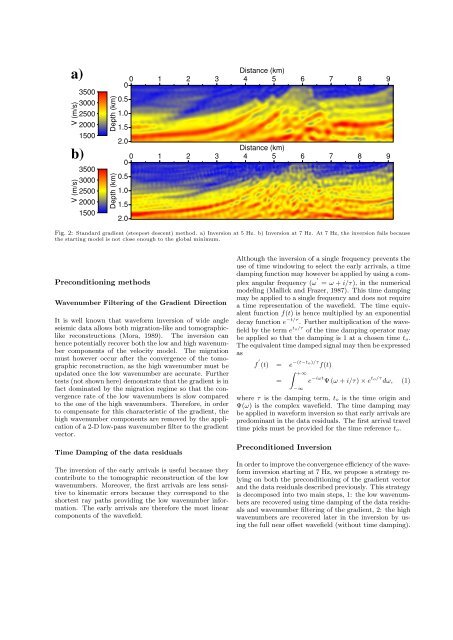
Fig. 2: Standard gradient (steepest descent) method. a) Inversion at 5 Hz. b) Inversion at 7 Hz. At 7 Hz, the inversion fails because
the starting model is not close enough to the global minimum.
Preconditioning methods
Wavenumber Filtering of the Gradient Direction
It is well known that waveform inversion of wide angle
seismic data allows both migration-like and tomographiclike
reconstructions (Mora, 1989). The inversion can
hence potentially recover both the low and high wavenumber
components of the velocity model. The migration
must however occur after the convergence of the tomographic
reconstruction, as the high wavenumber must be
updated once the low wavenumber are accurate. Further
tests (not shown here) demonstrate that the gradient is in
fact dominated by the migration regime so that the convergence
rate of the low wavenumbers is slow compared
to the one of the high wavenumbers. Therefore, in order
to compensate for this characteristic of the gradient, the
high wavenumber components are removed by the application
of a 2-D low-pass wavenumber filter to the gradient
vector.
Time Damping of the data residuals
The inversion of the early arrivals is useful because they
contribute to the tomographic reconstruction of the low
wavenumbers. Moreover, the first arrivals are less sensitive
to kinematic errors because they correspond to the
shortest ray paths providing the low wavenumber information.
The early arrivals are therefore the most linear
components of the wavefield.
Although the inversion of a single frequency prevents the
use of time windowing to select the early arrivals, a time
damping function may however be applied by using a complex
angular frequency (ω ′
= ω + i/τ), in the numerical
modeling (Mallick and Frazer, 1987). This time damping
may be applied to a single frequency and does not require
a time representation of the wavefield. The time equivalent
function f(t) is hence multiplied by an exponential
decay function e −t/τ . Further multiplication of the wavefield
by the term e to/τ of the time damping operator may
be applied so that the damping is 1 at a chosen time t o.
The equivalent time damped signal may then be expressed
as
f ′ (t) = e −(t−to)/τ f(t)
=
∫ +∞
−∞
e −iωt Ψ (ω + i/τ) × e to/τ dω, (1)
where τ is the damping term, t o is the time origin and
Ψ(ω) is the complex wavefield. The time damping may
be applied in waveform inversion so that early arrivals are
predominant in the data residuals. The first arrival travel
time picks must be provided for the time reference t o.
Preconditioned Inversion
In order to improve the convergence efficiency of the waveform
inversion starting at 7 Hz, we propose a strategy relying
on both the preconditioning of the gradient vector
and the data residuals described previously. This strategy
is decomposed into two main steps, 1: the low wavenumbers
are recovered using time damping of the data residuals
and wavenumber filtering of the gradient, 2: the high
wavenumbers are recovered later in the inversion by using
the full near offset wavefield (without time damping).