Sirgue, L., and Pratt, R. G., 2003. - Queen's University

Waveform Inversion under Realistic Conditions: Mitigation of non-linearity.
L. Sirgue, Ecole Normal Supérieure de Paris / CGG France, and R. Gerhard Pratt ∗ , Queen’s University,
Canada.
Summary
Using a realistic starting model and starting frequency,
standard waveform inversion methods are likely to fail to
converge to the global minimum of the misfit function. A
strategy that relies on the preconditioning of the gradient
direction and data residuals can be developed. Such
strategy can improve the convergence accuracy, but is
nevertheless delicate to implement.
Introduction
In waveform inversion, we aim to recover a quantitative
model of the subsurface in a way that minimizes the difference
between observed and calculated data. Because of
the high computational cost of calculating the synthetic
data, the inverse problem is the most often solved by local
methods which rely on the repeated calculation of the gradient
of the least-squares misfit function at each iteration
(Tarantola, 1984). Due to the high non-linearity of the
waveform inverse problem, the misfit function presents
numerous local minima that must be avoided in order
to insure convergence within the global minimum. The
success of waveform inversion of depends upon two main
aspects, 1: the accuracy of the starting model and 2:
the minimum frequency at which the inversion is initiated.
Often, synthetic examples of waveform inversion
are shown when both or one or these parameters are unrealistic
(Forgues et al., 1998; Freudenreich et al., 2001;
Sirgue and Pratt, 2001; Shipp and Singh, 2002), i.e. either
the starting model is unrealistically close to the true
model or the frequency is too low to be present in real
seismic data bandwidth.
In this paper we show that standard gradient methods
(without preconditioning) are unlikely to provide accurate
convergence if the starting model and the lowest frequency
are realistic. In such a case, a set of methods
for preconditioning of the gradient and the data residuals
must be applied in order to improve the convergence of
the waveform inversion.
We carry out our demonstration on a 2-D numerical experiment
in which the true model is an extended version
of the Marmousi model (18 km long). We first illustrate
the difficulties associate with inversion by showing a set
of inversions illustrating the issue of local minima. We
then propose a set of preconditioning operators that are
applied to the gradient and data residuals that improve
the convergence accuracy of the inversion.
a)
V (m/s)
b)
V (m/s)
3500
3000
2500
2000
1500
3500
3000
2500
2000
1500
Depth (km)
Depth (km)
0
0.5
1.0
1.5
2.0
0
0.5
1.0
1.5
2.0
Distance (km)
0 1 2 3 4 5 6 7 8 9
Distance (km)
0 1 2 3 4 5 6 7 8 9
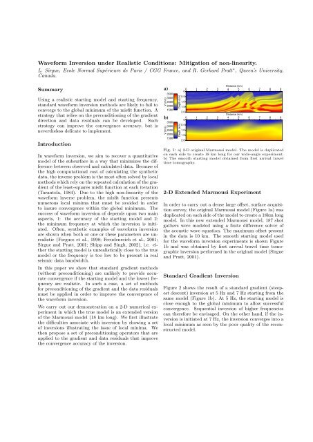
Fig. 1: a) 2-D original Marmousi model. The model is duplicated
on each side to create 18 km long for our wide-angle experiment.
b) The smooth starting model obtained from first arrival travel
time tomography.
2-D Extended Marmousi Experiment
In order to carry out a dense large offset, surface acquisition
survey, the original Marmousi model (Figure 1a) was
duplicated on each side of the model to create a 18km long
model. In this new extended Marmousi model, 187 shot
gathers were modeled using a finite difference solver of
the acoustic wave equation. The maximum offset present
in the data is 10 km. The smooth starting model used
for the waveform inversion experiments is shown Figure
1b and was obtained by first arrival travel time tomographic
inversion performed in the original model (Sirgue
and Pratt, 2001).
Standard Gradient Inversion
Figure 2 shows the result of a standard gradient (steepest
descent) inversion at 5 Hz and 7 Hz starting from the
same model (Figure 1b). At 5 Hz, the starting model is
close enough to the global minimum to allow successful
convergence. Sequential inversion of higher frequencies
can therefore be envisaged. On the other hand, if the inversion
is initiated at 7 Hz, the inversion converges into a
local minimum as seen by the poor quality of the reconstructed
model.

a)
V (m/s)
3500
3000
2500
2000
1500
b)
V (m/s)
3500
3000
2500
2000
1500
Depth (km)
Depth (km)
Distance (km)
0 1 2 3 4 5 6 7 8 9
0
0.5
1.0
1.5
2.0
0
0.5
1.0
1.5
2.0
Distance (km)
0 1 2 3 4 5 6 7 8 9
Fig. 2: Standard gradient (steepest descent) method. a) Inversion at 5 Hz. b) Inversion at 7 Hz. At 7 Hz, the inversion fails because
the starting model is not close enough to the global minimum.
Preconditioning methods
Wavenumber Filtering of the Gradient Direction
It is well known that waveform inversion of wide angle
seismic data allows both migration-like and tomographiclike
reconstructions (Mora, 1989). The inversion can
hence potentially recover both the low and high wavenumber
components of the velocity model. The migration
must however occur after the convergence of the tomographic
reconstruction, as the high wavenumber must be
updated once the low wavenumber are accurate. Further
tests (not shown here) demonstrate that the gradient is in
fact dominated by the migration regime so that the convergence
rate of the low wavenumbers is slow compared
to the one of the high wavenumbers. Therefore, in order
to compensate for this characteristic of the gradient, the
high wavenumber components are removed by the application
of a 2-D low-pass wavenumber filter to the gradient
vector.
Time Damping of the data residuals
The inversion of the early arrivals is useful because they
contribute to the tomographic reconstruction of the low
wavenumbers. Moreover, the first arrivals are less sensitive
to kinematic errors because they correspond to the
shortest ray paths providing the low wavenumber information.
The early arrivals are therefore the most linear
components of the wavefield.
Although the inversion of a single frequency prevents the
use of time windowing to select the early arrivals, a time
damping function may however be applied by using a complex
angular frequency (ω ′
= ω + i/τ), in the numerical
modeling (Mallick and Frazer, 1987). This time damping
may be applied to a single frequency and does not require
a time representation of the wavefield. The time equivalent
function f(t) is hence multiplied by an exponential
decay function e −t/τ . Further multiplication of the wavefield
by the term e to/τ of the time damping operator may
be applied so that the damping is 1 at a chosen time t o.
The equivalent time damped signal may then be expressed
as
f ′ (t) = e −(t−to)/τ f(t)
=
∫ +∞
−∞
e −iωt Ψ (ω + i/τ) × e to/τ dω, (1)
where τ is the damping term, t o is the time origin and
Ψ(ω) is the complex wavefield. The time damping may
be applied in waveform inversion so that early arrivals are
predominant in the data residuals. The first arrival travel
time picks must be provided for the time reference t o.
Preconditioned Inversion
In order to improve the convergence efficiency of the waveform
inversion starting at 7 Hz, we propose a strategy relying
on both the preconditioning of the gradient vector
and the data residuals described previously. This strategy
is decomposed into two main steps, 1: the low wavenumbers
are recovered using time damping of the data residuals
and wavenumber filtering of the gradient, 2: the high
wavenumbers are recovered later in the inversion by using
the full near offset wavefield (without time damping).

a)
V (m/s)
b)
V (m/s)
c)
V (m/s)
3500
3000
2500
2000
1500
3500
3000
2500
2000
1500
3500
3000
2500
2000
1500
Depth (km)
Depth (km)
Depth (km)
0
0.5
1.0
1.5
2.0
0
0.5
1.0
1.5
2.0
Distance (km)
0 1 2 3 4 5 6 7 8 9
0
0.5
1.0
1.5
2.0
Distance (km)
0 1 2 3 4 5 6 7 8 9
Distance (km)
0 1 2 3 4 5 6 7 8 9
Fig. 3: Preconditioned waveform inversion at 7 Hz. Stage 1: gradient wavenumber filtering is applied with a) τ = 0.1s and then b)
τ = 0.25s. b) Stage 2: Standard Inversion of offset 0.2-5 km. Each pass of stage 1 was carried out inverting from the near to the far
offsets.
a)
0
1
2
Offset (km)
-9 -8 -7 -6 -5 -4 -3 -2 -1 0 1 2 3 4 5 6 7 8
b)
0
1
2
Offset (km)
-9 -8 -7 -6 -5 -4 -3 -2 -1 0 1 2 3 4 5 6 7 8
Time (s)
3
4
5
6
7
Time (s)
3
4
5
6
7
Fig. 4: Time modeling using 114 frequencies. Shot point at 4.6 km. The source term is a Ricker with a peak frequency at 5 Hz.a)
The true dat. b) The modeling in the final model of inversion.

a) b)
Velocity (m/s)
1500 2000 2500 3000 3500 4000
c)
0
Velocity (m/s)
1500 2000 2500 3000 3500 4000
0
0
Velocity (m/s)
1500 2000 2500 3000 3500 4000
500
500
500
Depth (m)
1000
Depth (m)
1000
Depth (m)
1000
1500
1500
1500
2000
2000
2000
Fig. 5: Velocity traces showing the true model (gray), the starting model (dotted) and the inversion result (solid). a) Trace at 2.9
km.b) Trace at 4.5 km. c) Trace at 6 km.
For the recovery of the low wavenumbers, we advocate
an approach that inverts from the near to the far offset
data thus effectively carrying out a layer stripping
strategy (Figure 3a-c). The first arrival travel times were
picked in order to apply time damping with a initial value
of τ = 0.1 s. The wavenumber filter prevents wavenumbers
beyond k = 1 km −1 from being updated. The time
damping is then relaxed by decreasing the damping with
a value of τ = 0.25 s thus including later arrivals in the
inversion. The final stage of the inversion was carried out
with no preconditioning (Figure 3d), only the near offset
data were inverted. Although the modeling in time in the
final model (Figure 4b) shows an overall good fit with the
true data (Figure 4a), the velocity trace extracted from
the model (Figure 5) shows that some parts of the model
are less accurately recovered.
Conclusion
scheme:, in 63rd Mtg. Eur. Assn. of Expl. Geophys.,
Session: O–19.
Mallick, S., and Frazer, N. L., 1987, Practical aspects of
reflectivity modeling: Geophysics, 52, 1355–1364.
Mora, P., 1989, Inversion = migration + tomography:
Geophysics, 54, no. 12, 1575–1586.
Shipp, R. M., and Singh, S. C., 2002, Two-dimensional
full wavefield inversion of wide-aperture marine seismic
streamer data: Geophys. J. Int., 151, 325–344.
Sirgue, L., and Pratt, R., 2001, An optimal choice of temporal
frequencies for imaging: application to waveform
inversion.:, in 71st Ann. Internat. Mtg Soc. of Expl.
Geophys., 698–701.
Tarantola, A., 1984, Inversion of seismic reflection data
in the acoustic approximation: Geophysics, 49, no. 08,
1259–1266.
We have shown that when the starting frequency (7 Hz)
and the starting model used are both realistic, standard
waveform inversion is likely to fail. A set of preconditioning
tools should therefore be applied that improve the
convergence accuracy. However, the accuracy of the velocity
model may be difficult to evaluate on real data as
errors in the model will not be easy to identify.
Acknowledgments
We thank CGG France for sponsoring this work.
References
Forgues, E., Scala, E., and Pratt, R. G., 1998, High resolution
velocity model estimation from refraction and
reflection data:, in 68th Ann. Internat. Mtg, Soc. Expl.
Geophys., Expanded Abstracts Soc. of Expl. Geophys.,
1211–1214.
Freudenreich, Y., Singh, S., and Barton, P., 2001, Subbasalt
imaging using a full elastic wavefield inversion