Introduction to Computational Linguistics

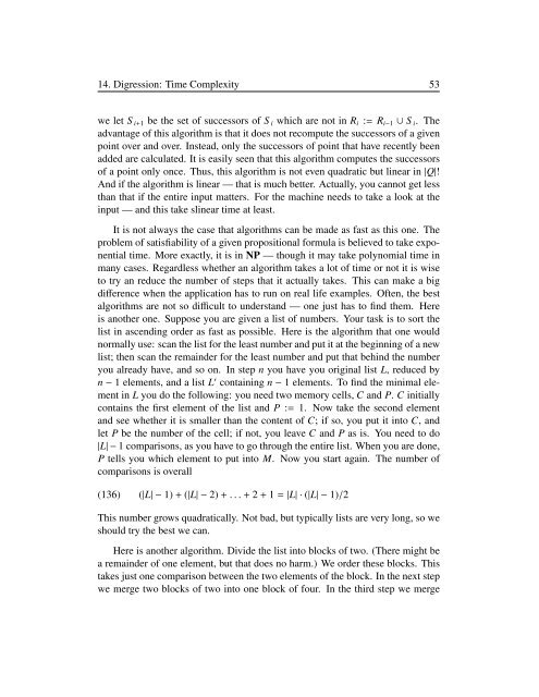
14. Digression: Time Complexity 53
we let S i+1 be the set of successors of S i which are not in R i := R i−1 ∪ S i . The
advantage of this algorithm is that it does not recompute the successors of a given
point over and over. Instead, only the successors of point that have recently been
added are calculated. It is easily seen that this algorithm computes the successors
of a point only once. Thus, this algorithm is not even quadratic but linear in |Q|!
And if the algorithm is linear — that is much better. Actually, you cannot get less
than that if the entire input matters. For the machine needs to take a look at the
input — and this take slinear time at least.
It is not always the case that algorithms can be made as fast as this one. The
problem of satisfiability of a given propositional formula is believed to take exponential
time. More exactly, it is in NP — though it may take polynomial time in
many cases. Regardless whether an algorithm takes a lot of time or not it is wise
to try an reduce the number of steps that it actually takes. This can make a big
difference when the application has to run on real life examples. Often, the best
algorithms are not so difficult to understand — one just has to find them. Here
is another one. Suppose you are given a list of numbers. Your task is to sort the
list in ascending order as fast as possible. Here is the algorithm that one would
normally use: scan the list for the least number and put it at the beginning of a new
list; then scan the remainder for the least number and put that behind the number
you already have, and so on. In step n you have you original list L, reduced by
n − 1 elements, and a list L ′ containing n − 1 elements. To find the minimal element
in L you do the following: you need two memory cells, C and P. C initially
contains the first element of the list and P := 1. Now take the second element
and see whether it is smaller than the content of C; if so, you put it into C, and
let P be the number of the cell; if not, you leave C and P as is. You need to do
|L| − 1 comparisons, as you have to go through the entire list. When you are done,
P tells you which element to put into M. Now you start again. The number of
comparisons is overall
(136) (|L| − 1) + (|L| − 2) + . . . + 2 + 1 = |L| · (|L| − 1)/2
This number grows quadratically. Not bad, but typically lists are very long, so we
should try the best we can.
Here is another algorithm. Divide the list into blocks of two. (There might be
a remainder of one element, but that does no harm.) We order these blocks. This
takes just one comparison between the two elements of the block. In the next step
we merge two blocks of two into one block of four. In the third step we merge