Takashi Yamano

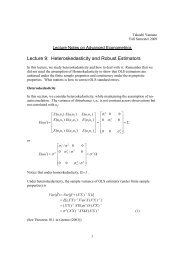
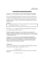
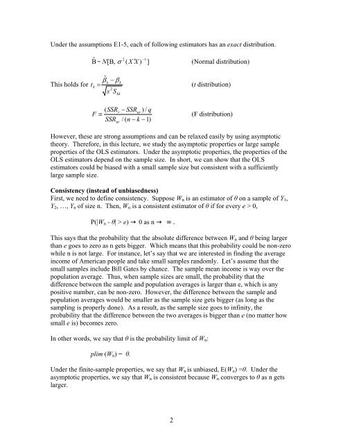
Under the assumptions E1-5, each of following estimators has an exact distribution.
ˆ 1
2 −
Β ~ N[
Β,
σ ( X ′ X ) ]
(Normal distribution)
This holds for
ˆ β − β
k k
t
k
=
(t distribution)
s 2 S
kk
F
( SSR
≡
SSR
r
ur
− SSR
ur
) / q
/ ( n − k −1)
(F distribution)
However, these are strong assumptions and can be relaxed easily by using asymptotic
theory. Therefore, in this lecture, we study the asymptotic properties or large sample
properties of the OLS estimators. Under the asymptotic properties, the properties of the
OLS estimators depend on the sample size. In short, we can show that the OLS
estimators could be biased with a small sample size but consistent with a sufficiently
large sample size.
Consistency (instead of unbiasedness)
First, we need to define consistency. Suppose W n is an estimator of θ on a sample of Y 1 ,
Y 2 , …, Y n of size n. Then, W n is a consistent estimator of θ if for every e > 0,
P(|W n - θ| > e) 0 as n
This says that the probability that the absolute difference between W n and θ being larger
than e goes to zero as n gets bigger. Which means that this probability could be non-zero
while n is not large. For instance, let’s say that we are interested in finding the average
income of American people and take small samples randomly. Let’s assume that the
small samples include Bill Gates by chance. The sample mean income is way over the
population average. Thus, when sample sizes are small, the probability that the
difference between the sample and population averages is larger than e, which is any
positive number, can be non-zero. However, the difference between the sample and
population averages would be smaller as the sample size gets bigger (as long as the
sampling is properly done). As a result, as the sample size goes to infinity, the
probability that the difference between the two averages is bigger than e (no matter how
small e is) becomes zero.
In other words, we say that θ is the probability limit of W n :
plim (W n ) = θ.
Under the finite-sample properties, we say that W n is unbiased, E(W n ) =θ. Under the
asymptotic properties, we say that W n is consistent because W n converges to θ as n gets
larger.
2