Dummy and Qualitative Dependent Variables

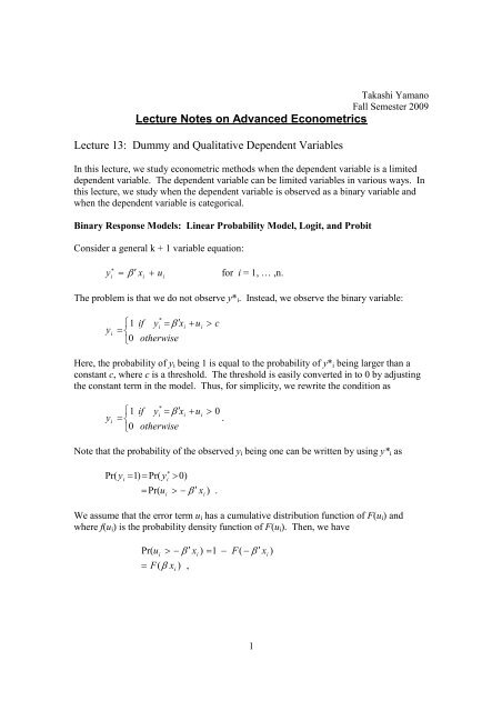
Takashi YamanoFall Semester 2009Lecture Notes on Advanced EconometricsLecture 13: Dummy and Qualitative Dependent VariablesIn this lecture, we study econometric methods when the dependent variable is a limiteddependent variable. The dependent variable can be limited variables in various ways. Inthis lecture, we study when the dependent variable is observed as a binary variable andwhen the dependent variable is categorical.Binary Response Models: Linear Probability Model, Logit, and ProbitConsider a general k + 1 variable equation:y = β ′ x + ufor i = 1, … ,n.∗iiiThe problem is that we do not observe y* i . Instead, we observe the binary variable:yi*⎧ 1 if y = ′iβ xi+ ui> c= ⎨⎩0otherwiseHere, the probability of y i being 1 is equal to the probability of y* i being larger than aconstant c, where c is a threshold. The threshold is easily converted in to 0 by adjustingthe constant term in the model. Thus, for simplicity, we rewrite the condition asyi*⎧ 1 if y = ′iβ xi+ ui> 0= ⎨.⎩0otherwiseNote that the probability of the observed y i being one can be written by using y* i as∗Pr( y = 1) = Pr( > 0)iy i= Pr( u > − β ′ x ) .iiWe assume that the error term u i has a cumulative distribution function of F(u i ) andwhere f(u i ) is the probability density function of F(u i ). Then, we havePr( u> − β ′ x ) = 1 − F(− β ′ x )i( xi= F β ) ,ii1

ecause the probability of u i being larger than − β ′ xiis the shaded area the left panel ofFigure 1. If the distribution has a symmetric shape, the shaded areas in the left panel areequal to the shaded area in the right panel of Figure 1.f(u i )1-F( − β′ x )F( β ′ x )− β ′x 00β ′ xFigure 1.If we replace the cumulative distribution function with the standard normal distributionfunction, then we have the Probit model.Probit: replace F β x ) with Φ ( β x )(iiΦ β x ) is the standard normal distribution.(iΦ(β ′ x)=∫β′x−∞φ(z)dz =∫β ′ x−∞1e2π2−z/ 2dzIf we we replace the cumulative distribution function with the logistic distribution, thenwe have the Logit model.Logit: replace F β x ) with Λ ( β x )(iiΛ β x ) is the logistic cumulative distribution function.(iΛ(e1+eβ ′ xβ ′ x)=β′x10.5 Λ ( β ′ x )0 β ′ x2

In the observations, we have n cases of zeros and ones with probability of F β x ) forones and − F(β x )1i(ifor zeros. Thus the joint probability or the likelihood function isorPr( y= 0, y= 1,..., y= 0) = Π [1 − F(β ′ x )] Π F(β ′ x )1 2niiyi= 0yi= 1L =Π[1− F(β ′ x )] [ F(β ′ x )]ii1−yi y iiTaking logs, we havelnL= Σ [(1 − y )ln(1 − F(β ′ x )) + y ln F(β ′ x )]iiiiiThis is the log likelihood. By differentiating ln L with respect to ∃, we get∂ ln L − f ( β ′ xi) xi(1 − yi) f ( β ′ xi) xiy= Σ{+∂ β i 1−F(β ′ x ) F(β ′ x )iii}[ y − F(β ′ x )]= ′ x ) x }iiΣ{ f ( βi [1−F(β ′ xi)] F(β ′ xi)∂ ln LThe maximum likelihood estimators are obtained at = 0.∂ βThus, we estimate this likelihood function to get β that maximizes the likelihoodfunction.Probit: ln L = Σ ln(1 − Φ(β ′ x )) + Σ ln Φ(β ′ x )yi= 0iyi= 1Logit: ln L = Σ ln(1 − Λ(β ′ x )) + Σ ln Λ(β ′ x )yi= 0iSimple Example of Logit modelConsider the following model:*yi= α + β di+ uiy = 1 if y* > 0y = 0 otherwiseAs we studied in the class, the log likelihood function isln L = Σ [(1 − y )ln(1 − F(β ′ x )) + y ln F(β ′ x )](1)iiyi= 1Now, replace the cumulative function with the logistic function:iiiiiii3

Fe1 + ee1 + eβ ' xα + β d( β ' x)= Λ(β ' x)= =β ' xα + β d(a)(b)Write down the log likelihood function (1) with the logistic function.Suppose you have the data of 10 observations:Y0 1d 0 3 71 0 0Show that in this case, the log likelihood function becomesαln L = 7α− 10ln (1 + e )(2)(c)(d)(e)By differentiating the log likelihood function (2) w.r.t. ∀, find ∀ thatααmaximizes the log likelihood function. (Hint: ∂ e / ∂α= e )By using the data called MLE.dta, estimate the model and confirm youranswer.Suppose you have the data of 10 observations:dY0 10 2 31 1 4Find ˆ α and ˆ β by the same method in (a)–(d). Show me how you obtainthe estimators.The Likelihood Ratio TestLR = - 2[ln L r - ln L ur ]This is like a F-test for the maximum likelihood estimation. Note that in maximumlikelihood estimation, we want to maximize the likelihood, instead of minimizing (theleast square). Thus the larger the better (remember however that the likelihood is anegative number), thus the likelihood of the unrestricted model, ln L ur , will be larger thanthe restricted model, ln L r . Thus the inside the bracket will be negative, and LR will bepositive. If LR is a large number: if there is a significant difference in ln L r and ln L ur ,then the additional variables in the unrestricted model are jointly significant.4

Measuring the Goodness of FitThe percent correctly predicted: define∗∗∗yˆ i= 1 if yi> 0.5 and yˆi= 1otherwiseand create a 2 by 2 matrix. And calculate a percentage of correct prediction on both y i = 1and y i = 0.Alternatively you can get a pseudo R-squared:Pseudo R-squared = 1 - ln L/ ln L 0ln L 0 is the log likelihood from a model with the constant term only.Example 13-1: Food Aid Targeting in Ethiopia (Jayne et al., 2002). ***** WEREDA LEVEL ANALYSIS *****;. *** Food for Free ****;. probit wvfreed;Probit estimates Number of obs = 343LR chi2(0) = -0.00Prob > chi2 = .Log likelihood = -200.44456 Pseudo R2 = -0.0000------------------------------------------------------------------------------wvfreed | Coef. Std. Err. z P>|z| [95% Conf. Interval]-------------+----------------------------------------------------------------_cons | -.6093778 .0724429 -8.41 0.000 -.7513633 -.4673923------------------------------------------------------------------------------. probit wvfreed teg am oro other lpcninc elev> shrtplot overplot diseplot;Probit estimates Number of obs = 343LR chi2(9) = 79.36Prob > chi2 = 0.0000Log likelihood = -160.76343 Pseudo R2 = 0.1980------------------------------------------------------------------------------wvfreed | Coef. Std. Err. z P>|z| [95% Conf. Interval]-------------+----------------------------------------------------------------Tigray | 1.467662 .3326602 4.41 0.000 .8156605 2.119664Amhara | .1965025 .2465459 0.80 0.425 -.2867187 .6797236Oromiya | -.1079401 .2379339 -0.45 0.650 -.5742821 .3584018Other | .8938703 .3946693 2.26 0.024 .1203327 1.667408Ln(pc inc)| -.4626233 .1515389 -3.05 0.002 -.7596341 -.1656125Elevation | .0340291 .017033 2.00 0.046 .000645 .0674132Shortage | .0200977 .0050222 4.00 0.000 .0102542 .02994115

Flood | .012639 .0071791 1.76 0.078 -.0014317 .0267098Insect | .0070072 .0078859 0.89 0.374 -.0084488 .0224632_cons | .8524934 .8673863 0.98 0.326 -.8475525 2.552539------------------------------------------------------------------------------** This is a Wald test ************;. test shrtplot overplot diseplot;( 1) shrtplot = 0.0( 2) overplot = 0.0( 3) diseplot = 0.0chi2( 3) = 17.59Prob > chi2 = 0.0005** Log Likelihood Test, obtaining the log likelihood from unrestricted model;. lrtest, saving(0);** Obtaining the percent correctly predicted *****. predict y1;(option p assumed; Pr(wvfreed)). gen y1_one=(y1>0.5);. tab wvfreed y1_one, row;| y1_onewvfreed | 0 1 | Total-----------+----------------------+----------0 | 235 15 | 250| 94.00 6.00 | 100.00-----------+----------------------+----------1 | 59 34 | 93| 63.44 36.56 | 100.00-----------+----------------------+----------Total | 294 49 | 343| 85.71 14.29 | 100.00*** Restricted Model;. probit wvfreed teg am oro other lpcninc elev;Probit estimates Number of obs = 343LR chi2(6) = 60.99Prob > chi2 = 0.0000Log likelihood = -169.9489 Pseudo R2 = 0.1521------------------------------------------------------------------------------wvfreed | Coef. Std. Err. z P>|z| [95% Conf. Interval]-------------+----------------------------------------------------------------teg | 1.679131 .3217638 5.22 0.000 1.048485 2.309776am | .349624 .2339933 1.49 0.135 -.1089944 .8082424oro | -.0745053 .2318984 -0.32 0.748 -.5290178 .3800072other | .8442578 .3812492 2.21 0.027 .0970232 1.591492lpcninc | -.5494286 .146091 -3.76 0.000 -.8357616 -.2630956elev | .0264549 .0163385 1.62 0.105 -.0055679 .0584778_cons | 1.716908 .8199178 2.09 0.036 .1098989 3.323918------------------------------------------------------------------------------**** Log likelihood test *************;. lrtest;Probit: likelihood-ratio test chi2(3) = 18.37Prob > chi2 = 0.0004End of Example 13-16

Marginal EffectsThe coefficients of Probit or Logit in likelihood function do not represent changes inprobabilities. To get effects on marginal probability, we need to transform the estimatedcoefficient.The probability model isE y]= 0 [1 − F(β ′ x )] + 1 [ F(β ′ x )][ii= F( β ′ xi)Thus, the marginal changes in the probability is, by using the chain rule,∂ E [ y]⎛ d F(β ′ x)⎞ d(β x)=′x⎜d(β x)⎟∂ ⎝ ′ ⎠ dx= f β ′ x ) β .(iFor Probit and Logit, we have∂ E[y]∂x=∂ E[y]∂x= Λ′ xProbit: φ ( β ) βLogit : ( β x)( 1 − Λ(β x)) βEvaluate at means:∂ E[y]∂x∂ E[y]∂xProbit: = φ ( β x) βLogit : = Λ ( β x)( 1 − Λ(β x)) βChanges in Probability when a Change in x is Not So Marginal′′′Because Probit and Logit are no-linear model, a marginal change (which is a linearapproximation at some point) can be misleading. Thus, we need to conduct a simulation.Suppose we want to know a change in the probability of y i = 1 when x s changes from a tob:Pr (y i =1| x s = b ) - Pr (y i =1| x s = a )See the next example.′′7

Example 13-2: Food Aid Targeting in Ethiopia (Jayne et al., 2002)dprobit: Marginal Probability Model. dprobit wvfreed teg am oro other lpcninc elev> shrtplot overplot diseplot;Iteration 0: log likelihood = -200.44456Iteration 1: log likelihood = -161.75807Iteration 2: log likelihood = -160.76658Iteration 3: log likelihood = -160.76343Probit estimates Number of obs = 343LR chi2(9) = 79.36Prob > chi2 = 0.0000Log likelihood = -160.76343 Pseudo R2 = 0.1980------------------------------------------------------------------------------wvfreed | dF/dx Std. Err. z P>|z| x-bar [ 95% C.I. ]---------+--------------------------------------------------------------------teg*| .5347784 .1071274 4.41 0.000 .090379 .324813 .744744am*| .0632314 .081563 0.80 0.425 .268222 -.096629 .223092oro*| -.0334596 .0731175 -0.45 0.650 .405248 -.176767 .109848other*| .331359 .1537268 2.26 0.024 .046647 .03006 .632658lpcninc | -.1444777 .0471902 -3.05 0.002 5.80889 -.236969 -.051987elev | .0106273 .0053209 2.00 0.046 20.4433 .000199 .021056shrtplot | .0062765 .0015886 4.00 0.000 7.34191 .003163 .00939overplot | .0039472 .0022367 1.76 0.078 4.51159 -.000437 .008331diseplot | .0021883 .0024627 0.89 0.374 7.34973 -.002638 .007015---------+--------------------------------------------------------------------obs. P | .271137pred. P | .2420307 (at x-bar)------------------------------------------------------------------------------(*) dF/dx is for discrete change of dummy variable from 0 to 1z and P>|z| are the test of the underlying coefficient being 0**** Predict at means;. predict ymean;(option p assumed; Pr(wvfreed))*** Get summary of log(per capita income);. su lpcninc, d;(mean) lpcninc-------------------------------------------------------------Percentiles Smallest1% 4.339287 3.5194915% 4.836071 3.98048310% 5.108971 4.324318 Obs 34325% 5.446068 4.339287 Sum of Wgt. 34350% 5.863084 Mean 5.808894Largest Std. Dev. .578566575% 6.182746 6.98703690% 6.546782 7.029579 Variance .334739295% 6.76193 7.078065 Skewness -.339784499% 6.987036 7.130215 Kurtosis 3.4257688

*** A Simulation in Pr(y) when lnpcninc changes from 25 th to 75 th percentile;** Set the lpnninc at 25 th percentile;. replace lpcninc=5.446;(343 real changes made)** Predict at Pr(y) at 25 th , holding other variables at means;. predict yat25;(option p assumed; Pr(wvfreed))** Set the lpnninc at 75 th percentile;. replace lpcninc=6.813;(343 real changes made)** Predict at Pr(y) at 75 th , holding other variables at means;. predict yat75;(option p assumed; Pr(wvfreed)). su ymean yat25 yat75;Variable | Obs Mean Std. Dev. Min Max-------------+-----------------------------------------------------ymean | 343 .2713801 .2179637 .0246233 .9457644yat25 | 343 .312233 .2115653 .0845005 .9469762yat75 | 343 .1599189 .1798231 .0223308 .8373954End of Example 12Fixed Effects Logit ModelA fixed effects Logit model that accounts for the heterogeneity ise1+eαi+β′xitPr ( yit=1) =α + βx,iitwhere α is the fixed effect for observation i. For simplicity, we only consider cases foriT = 2. The unconditional likelihood isL = Π Pr( Yi1 = yi1)Pr(Yi2= yi2),iwhere y it is the value that Y it takes at time t for observation i. (The likelihood is theproduct of the probabilities because the observations are independent.) The sum of Y i1and Y i2 can take three values: 0, 1, and 2. When the sum is zero, there is only onecombination (Y i1, Y i2 ) = (0, 0). When the sum is two, there is also one combination: (Y i1,Y i2 ) = (1, 1). In these two cases, we do learn nothing about the attributes for x i on Y itbecause there is no variation in Y it . Observations with these combinations will bedropped from the analysis.When the sum is one, there are two possibilities: (Y i1, Y i2 ) = (1, 0) and (0, 1). Thus, wehave9

Pr(0,1)Pr(0,1| sum = 1) =, orPr(0,1) + Pr(1,0)Pr(1,0)Pr(1,0 | sum = 1) =.Pr(0,1) + Pr(1,0)The conditional probability by using logit functions isPr(1) Pr(0)Pr(0) Pr(1) + Pr(1) Pr(0)=1α11+e+ β′xi1α1e1+eα1+e1+e+ β′x11β′xi 2i1α + β′xα + β′xi 2=i11α11+eα1+e+1+e+ β′x2β′x1i1α + β′x11α11+e+ β′xi 2α1+ β ′ xi1β ′ x1=′′=′ ′=α + β x α + β x β x β x β ′(x − xe1ei 2+ e1i1ee+ ei 2i1ei 21i1)+ 1= 1− Λ[β ′(xi2 − xi1)]Thus, in the fixed effects logit model, the fixed effect, α , is eliminated. Similarly, theiPr(1)Pr(0)1= 1−′( x 2 − 1Pr(0)Pr(1) + Pr(1)Pr(0)) i xie β + 1= Λ β ′(x − x )] .[i2 i1Thus, the log likelihood function for observation i isL = [ sum = 1]{ w ln( Λ(β ∆′ x ) + (1 − w )ln(1 − Λ(∆x))}i1iiiiwhere w i = 1 if (Y i1, Y i2 ) = (0, 1) and w i = 0 if (Y i1, Y i2 ) = (1, 0).The estimated coefficients of the fixed effects logit model can be interpreted as theeffects on log-odd ratio. But we are unable to find level effects of x i on the dependentvariables. This is partly the reasons that some researchers use the (liner) fixed effectsmodel on the binary response dependent variables to control for fixed effects.10

Multinomial Logit ModelThe logit model for binary response can be extended for more than two outcomes that arenot ordered. Let y denote a random variable taking on the values [0, 1, …, J]. Since theprobabilities must sum to unity, Pr(y = 0| x) is determined once we know the probabilitiesfor j = 1, …, J. Therefore, the probability that y takes j can be written asPr( YiPr( Yie= j)=J1+= 0) =1+β ′ xj∑k = 1J1∑k = 1ieeβ ′ xkifor j = 1,..., Jfor j = 0β ′ x.ki, andNote that for a binary response case, J = 2, this becomes the logit model. The modelimplies that we can compute J log-odd ratiosPijln[ ] = β ′jxi.Pi0This implies that the estimated coefficients of the Multinomial Logit should beinterpreted as the effects on the log-off ratios of choice j and the base choice, j = 0.The marginal effects on the particular outcome are∂Pj∂xi∑= P [ β − P β ].jjJk=1kkNote that this result suggests that the direction of the marginal effect could be differentfrom the sign of the estimated coefficient (of the odd-ratio).Quiz: Show that the sum of the marginal effects for all outcomes is zero.(STATA 9 provides the marginal effects.)Example 13-3: Primary and Secondary School Choice among Female Orphans and Nonorphansin Uganda (Yamano, Shimamura, and Sserunkuuma, 2005, EDCC, vol. 54 (4):833-856, Table 9)In this example, the dependent variable is a choice variable: Not attending school,attending primary school, and attending secondary school. The focus is on orphans who11

lost at least one parent before reaching 15 years old. The sample in this example includegirls aged 15 to 18.. xi: mlogit type oneporp vdorphan onepnorp bothout age16 age17 age18 fhhedumen eduwomen eldmale eldfmale wkmen wkwomen llsize lprop i.distcode ifsex==2, base(0)i.distcode _Idistcode_12-40 (naturally coded; _Idistcode_12 omitted)Multinomial logistic regression Number of obs = 384LR chi2(88) = 247.35Prob > chi2 = 0.0000Log likelihood = -279.30422 Pseudo R2 = 0.3069------------------------------------------------------------------------------type | Coef. Std. Err. z P>|z| [95% Conf. Interval]-------------+----------------------------------------------------------------Primary SchoolSingleOrphans| -.67788 .7392469 -0.92 0.359 -2.126777 .7710173DoubleOrphans| -1.382794 .6558163 -2.11 0.035 -2.66817 -.0974173One parent | 1.047395 .7657416 1.37 0.171 -.4534311 2.548221No parents | -1.347218 .6773663 -1.99 0.047 -2.674832 -.0196047age16 | -2.014747 .4909821 -4.10 0.000 -2.977054 -1.05244age17 | -1.864725 .5329909 -3.50 0.000 -2.909368 -.8200819age18 | -4.219341 .6813643 -6.19 0.000 -5.554791 -2.883892Female headed| .1620776 .6449858 0.25 0.802 -1.102071 1.426226edumen | -.0605027 .0656405 -0.92 0.357 -.1891557 .0681504eduwomen | -.1250235 .0888526 -1.41 0.159 -.2991714 .0491244eldmale | 1.613167 .6189866 2.61 0.009 .3999752 2.826358eldfmale | .1462345 .673432 0.22 0.828 -1.173668 1.466137wkmen | -.030326 .2035947 -0.15 0.882 -.4293643 .3687124wkwomen | -.1877117 .1806674 -1.04 0.299 -.5418134 .16639log(Landsize)| .0680674 .2684975 0.25 0.800 -.458178 .5943128log(assets) | .3132038 .1841006 1.70 0.089 -.0476267 .6740342_Idistcod~13 | .5352554 1.158086 0.46 0.644 -1.734552 2.805062_Idistcod~40 | -39.98424 3.19e+08 -0.00 1.000 -6.26e+08 6.26e+08_cons | -.2099659 2.205778 -0.10 0.924 -4.533211 4.113279-------------+----------------------------------------------------------------Secondary SchoolSingleOrphans| -.960672 .6962642 -1.38 0.168 -2.325325 .4039808Doubleorphans| -2.159722 .6353289 -3.40 0.001 -3.404944 -.9145006One parent | -.9110557 .816869 -1.12 0.265 -2.512089 .689978No parents | -1.975631 .6386655 -3.09 0.002 -3.227393 -.72387age16 | -.4085832 .5078172 -0.80 0.421 -1.403886 .5867202age17 | -.093862 .5384703 -0.17 0.862 -1.149244 .9615205age18 | -.7141053 .5384291 -1.33 0.185 -1.769407 .3411964Female headed| .5078927 .5961982 0.85 0.394 -.6606342 1.67642edumen | -.0067266 .0619717 -0.11 0.914 -.128189 .1147357eduwomen | .115019 .0816583 1.41 0.159 -.0450284 .2750663eldmale | .9500993 .609837 1.56 0.119 -.2451593 2.145358eldfmale | .6985087 .6432948 1.09 0.278 -.5623261 1.959343wkmen | -.1848425 .1923146 -0.96 0.336 -.5617723 .1920873wkwomen | -.5618054 .1758088 -3.20 0.001 -.9063843 -.2172265log(Landsize)| .4230313 .2572931 1.64 0.100 -.081254 .9273165log(assets) | .4838305 .1805556 2.68 0.007 .129948 .837713_Idistcod~13 | -.2492886 1.210194 -0.21 0.837 -2.621225 2.122648_Idistcod~40 | -.3812108 1.052142 -0.36 0.717 -2.443371 1.680949_cons | -5.631196 2.233789 -2.52 0.012 -10.00934 -1.253051------------------------------------------------------------------------------(Outcome type==0 is the comparison group)12