Takashi Yamano

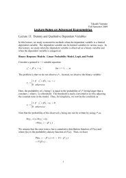
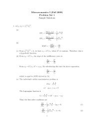
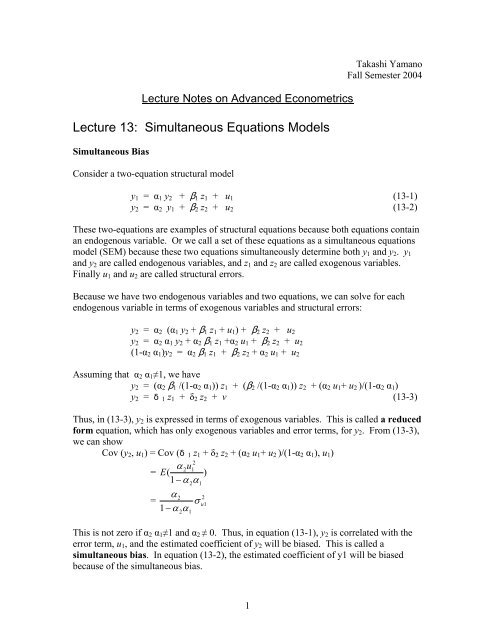
Lecture Notes on Advanced EconometricsLecture 13: Simultaneous Equations ModelsSimultaneous BiasConsider a two-equation structural modelTakashi YamanoFall Semester 2004y 1 = α 1 y 2 + $ 1 z 1 + u 1 (13-1)y 2 = α 2 y 1 + $ 2 z 2 + u 2 (13-2)These two-equations are examples of structural equations because both equations containan endogenous variable. Or we call a set of these equations as a simultaneous equationsmodel (SEM) because these two equations simultaneously determine both y 1 and y 2 . y 1and y 2 are called endogenous variables, and z 1 and z 2 are called exogenous variables.Finally u 1 and u 2 are called structural errors.Because we have two endogenous variables and two equations, we can solve for eachendogenous variable in terms of exogenous variables and structural errors:y 2 = α 2 (α 1 y 2 + $ 1 z 1 + u 1 ) + $ 2 z 2 + u 2y 2 = α 2 α 1 y 2 + α 2 $ 1 z 1 +α 2 u 1 + $ 2 z 2 + u 2(1-α 2 α 1 )y 2 = α 2 $ 1 z 1 + $ 2 z 2 + α 2 u 1 + u 2Assuming that α 2 α 1 ≠1, we havey 2 = (α 2 $ 1 /(1-α 2 α 1 )) z 1 + ($ 2 /(1-α 2 α 1 )) z 2 + (α 2 u 1 + u 2 )/(1-α 2 α 1 )y 2 = 1 z 1 + δ 2 z 2 + v (13-3)Thus, in (13-3), y 2 is expressed in terms of exogenous variables. This is called a reducedform equation, which has only exogenous variables and error terms, for y 2 . From (13-3),we can showCov (y 2 , u 1 ) = Cov ( 1 z 1 + δ 2 z 2 + (α 2 u 1 + u 2 )/(1-α 2 α 1 ), u 1 )2α2u1= E ( )1−αα=α21−αα2212σ u 11This is not zero if α 2 α 1 ≠1 and α 2 ≠ 0. Thus, in equation (13-1), y 2 is correlated with theerror term, u 1 , and the estimated coefficient of y 2 will be biased. This is called asimultaneous bias. In equation (13-2), the estimated coefficient of y1 will be biasedbecause of the simultaneous bias.1

In this case, we can not identify either curve, because z is included in the both equations.Thus, z does not satisfy the exclusion restrictions. This is illustrated in Panel 2. Weobserve changes in price and quantity from A to C. But, because both curves can shiftfrom A to C, we can not trace curves. Both curves in Panel 2 could be steeper or flatter.Reduced Form Equations in General CasesIn general, we can have more than two simultaneous equations (more than twoendogenous variables) at once. Suppose there are 3-endogenous variables:y 1 = f 1 (y 2 , y 3 , z 1 ,z 2 , z 3 , z 4 )y 2 = f 2 (y 1 , y 3 , z 1 , z 2 , z 5 , z 6 , z 7 )y 3 = f 3 (y 1 , y 2 , z 1 , z 2 , z 8 , z 9 , z 10 )The reduced form equation for each endogenous variable will contain all of theexogenous variables:y 1 = f 1 (z 1 ,z 2 , z 3 , z 4 , z 5 , z 6 , z 7 , z 8 , z 9 , z 10 )y 2 = f 2 (z 1 ,z 2 , z 3 , z 4 , z 5 , z 6 , z 7 , z 8 , z 9 , z 10 )y 3 = f 3 (z 1 ,z 2 , z 3 , z 4 , z 5 , z 6 , z 7 , z 8 , z 9 , z 10 )From these reduced form equations, we can identify endogenous variables in thestructural from equations.Example 13-1: Inflation and Openness by using Openness.dtaSee Example 16.4 and 16.6 in Wooldridge:The Reduced Form Equation for “Open”. reg open lpcinc llandSource | SS df MS Number of obs = 114-------------+------------------------------ F( 2, 111) = 45.17Model | 28606.1936 2 14303.0968 Prob > F = 0.0000Residual | 35151.7966 111 316.682852 R-squared = 0.4487-------------+------------------------------ Adj R-squared = 0.4387Total | 63757.9902 113 564.230002 Root MSE = 17.796------------------------------------------------------------------------------open | Coef. Std. Err. t P>|t| [95% Conf. Interval]-------------+----------------------------------------------------------------lpcinc | .5464812 1.49324 0.37 0.715 -2.412473 3.505435lland | -7.567103 .8142162 -9.29 0.000 -9.180527 -5.953679_cons | 117.0845 15.8483 7.39 0.000 85.68006 148.489------------------------------------------------------------------------------The OLS for inflation. reg inf open lpcincSource | SS df MS Number of obs = 114-------------+------------------------------ F( 2, 111) = 2.63Model | 2945.92812 2 1472.96406 Prob > F = 0.07643

Residual | 62127.4936 111 559.70715 R-squared = 0.0453-------------+------------------------------ Adj R-squared = 0.0281Total | 65073.4217 113 575.870989 Root MSE = 23.658------------------------------------------------------------------------------inf | Coef. Std. Err. t P>|t| [95% Conf. Interval]-------------+----------------------------------------------------------------open | -.2150695 .0946289 -2.27 0.025 -.402583 -.027556lpcinc | .0175683 1.975267 0.01 0.993 -3.896555 3.931692_cons | 25.10403 15.20522 1.65 0.102 -5.026122 55.23419------------------------------------------------------------------------------The 2SLS for inflation. ivreg inf (open= lland) lpcincInstrumental variables (2SLS) regressionSource | SS df MS Number of obs = 114-------------+------------------------------ F( 2, 111) = 2.79Model | 2009.22775 2 1004.61387 Prob > F = 0.0657Residual | 63064.194 111 568.145892 R-squared = 0.0309-------------+------------------------------ Adj R-squared = 0.0134Total | 65073.4217 113 575.870989 Root MSE = 23.836------------------------------------------------------------------------------inf | Coef. Std. Err. t P>|t| [95% Conf. Interval]-------------+----------------------------------------------------------------open | -.3374871 .1441212 -2.34 0.021 -.6230728 -.0519014lpcinc | .3758247 2.015081 0.19 0.852 -3.617192 4.368841_cons | 26.89934 15.4012 1.75 0.083 -3.619161 57.41783------------------------------------------------------------------------------Instrumented: openInstruments: lpcinc lland------------------------------------------------------------------------------The estimated coefficient changes from -0.215 to -0.337. There is no overidentificationproblem because the number of endogenous variable and theinstrument is both one.4