Microeconomics I (Fall 2009) Problem Set 1 Sample Solutions

Microeconomics I (Fall 2009)
Problem Set 1
Sample Solutions
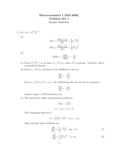
1. u(x 1 , x 2 ) = x 1/2
1 x 1/2
2 .
(a)
(b)
MU 1 = ∂u(x 1, x 2 )
∂x 1
= 1 2 x− 1 2
1 x 1 2
2 .
MU 2 = ∂u(x 1, x 2 )
∂x 2
= 1 2 x 1 2
1 x − 1 2
2 .
MRS = − MU 1
MU 2
= − x 2
x 1
.
(c) From x 1/2
1 x 1/2
2 = k, we have x 2 = k 2 /x 1 , where k 2 is constant. Therefore, this is
a hyperbolic function.
(d) From x 2 = k 2 /x 1 , the slope of the indifference curve is:
dx 2
= − k2
.
dx 1
From x 2 = k 2 /x 1 , k 2 = x 1 x 2 . By substituting this into the above expression,
which is equal to MRS derived in (b).
x 2 1
dx 2
dx 1
= − x 2
x 1
,
(e) The individual’s utility maximization problem is:
Max x 1 2
1 x 1 2
2
The Lagrangian function is
s.t.
p 1 x 1 + x 2 = Y
Thus, the first-order conditions are
L = x 1 2
1 x 1 2
2 + λ(Y − p 1 x 1 − x 2 )
∂L
∂x 1
= 1 2 x− 1 2
1 x 1 2
2 − λp 1 = 0, (1)
∂L
∂x 2
= 1 2 x 1 2
1 x − 1 2
2 − λ = 0. (2)
1

By dividing (1) by (2), we have x 2 /x 1 = p 1 , or x 2 = p 1 x 1 . By substituting this
into the budget constraint, the demand functions for goods 1 and 2 are given by
x 1 = Y
2p 1
,
x 2 = Y 2 .
Note that the demand function for good 1 is again hyperbolic.
2. u(x 1 , x 2 ) = min{2x 1 , x 2 }.
(a) (Omitted. Please refer to Figure 4.4 (b) on p. 82 in the textbook for the case of
u(x 1 , x 2 ) = min{x 1 , x 2 }.)
(b) Let us consider a point (x 0 1, x 0 2) on x 2 = 2x 1 . Then, x 0 2 = 2x 0 1 (or equivalently
x 0 1 = x 0 2/2) holds.
i. (x 1 , x 2 ) = (x 1 , x 0 2), x 1 > x 0 2/2: In this case, from 2x 1 > x 0 2, we have
u(x 1 , x 2 ) = min{2x 1 , x 0 2} = x 0 2. An increase in x 1 , therefore, does not raise
utility. Thus, MU 1 = 0. On the other hand, MU 2 = ∂u(x 1 , x 2 )/∂x 2 =
∂x 2 /∂x 2 = 1. Thus, MRS = −MU 1 /MU 2 = 0.
ii. (x 1 , x 2 ) = (x 0 1, x 2 ), x 2 > x 0 2: Since x 2 > x 0 2 = 2x 0 1, u(x 0 1, x 2 ) = min{2x 0 1, x 2 } =
2x 0 1. From ∂u(x 1 , x 2 )/∂x 2 = ∂(2x 1 )/∂x 2 = 0, MU 2 = 0. Besides, from
∂u(x 1 , x 2 )/∂x 1 = ∂(2x 1 )/∂x 1 = 2, MU 1 = 2. Therefore, MRS = −2/0 =
−∞.
iii. (x 1 , x 2 ) = (x 0 1, x 0 2): In this case, MRS is not defined.
(c) Rearranging the budget constraint, p 1 x 1 + x 2 = Y , gives x 2 = Y − p 1 x 1 . From the
shape of indifference curves, it is inferred that utility is maximized on x 2 = 2x 1 .
Solving the simultaneous equations,
x 1 (p 1 ) =
x 2 (p 1 ) =
Y
p 1 + 2 ,
2Y
p 1 + 2 .
You already know how to depict the graph of x 1 (p 1 ).
3. u(x 1 , x 2 ) = x 1 + x 2 .
(a)
MRS = − MU 1
MU 2
= −1.
(3)
2

(b) By rearranging the budget constraint, x 2 = Y − p 1 x 1 . Note that the slope of the
budget line is −p 1 while the slope of indifference curves is −1.
i. If p 1 > 1, utility is maximized at (x 1 , x 2 ) = (0, Y ). That is, the whole income
is spent on good 2. This is because the individual is indifferent between goods
1 and 2, and because the price of good 2 (p 2 = 1) is lower than that of good
1 (p 1 > 1).
ii. By contrast, if p 1 < 1, the individual spends the whole income on good 1.
The demand for good 1 is thus x 1 = Y/p 1 .
iii. Lastly, if p 1 = 1, the prices of goods 1 and 2 are identical. Therefore, the
demand for good 1 could be any amount between 0 and Y.
In summary, the demand function for good 1 is:
⎧
⎨ Y/p 1 if p 1 < 1
x 1 (p 1 ) = 0 if p 1 > 1
⎩
any value between 0 and Y if p 1 = 1
3