Takashi Yamano

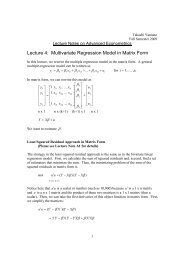
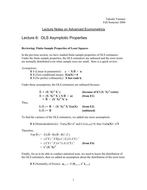
Lecture Notes on Advanced Econometrics
Lecture 6: OLS Asymptotic Properties
Takashi Yamano
Fall Semester 2004
Reviewing: Finite-Sample Properties of Least Squares
In the previous section, we have studied finite-sample properties of OLS estimators.
Under the finite-sample properties, the OLS estimators are unbiased and the error terms
are normally distributed even when sample sizes are small. Here is a quick review:
Assumptions:
E 1 (Linear in parameters): y = X % + u
E 2 (Zero conditional mean): E(u|X) = 0
E 3 (No perfect collinearity): X has rank k.
Under these assumptions, the OLS estimators are unbiased because:
Thus,
Βˆ = (XtX) -1 Xty
(because of E3 (XtX) -1 exists)
Βˆ = (XtX) -1 Xt( X % + u) (from E1)
= % + (XtX) -1 Xtu
E( Β ˆ ) = % + (XtX)
XtE(u|X) (from E2)
E(Β ˆ ) = %
(unbiased)
To find the variance of the OLS estimators, we added one more assumptioin.
E 4 (Homoskedasticity): Var(u i |X)=F 2 and Cov(u i ,u j )=0, thus Var(u|X)= F 2 I
Therefore,
Var( Β ˆ ) = E [(
Βˆ
−Β)(
Βˆ
− Β)
′ | X ]
− 1
−1
= ( X ′X ) X ′ E[
u u′
| X ] X ( X ′ X )
− 1 2
−1
= ( X ′X ) X ′(
σ I)
X ( X ′ X ) (from E4)
= F 2 (XtX) -1
Finally, for us to be able to conduct statistical tests, we need to know the distribution of
the OLS estimators, then we added an assumption about the distribution of the error term:
E 5 (Normality of Errors): u n x 1 ~ N (0 n x 1, F 2 I n x n )
1

Under the assumptions E1-5, each of following estimators has an exact distribution.
ˆ 1
2 −
Β ~ N[
Β,
σ ( X ′ X ) ]
(Normal distribution)
This holds for
ˆ β − β
k k
t
k
=
(t distribution)
s 2 S
kk
F
( SSR
≡
SSR
r
ur
− SSR
ur
) / q
/ ( n − k −1)
(F distribution)
However, these are strong assumptions and can be relaxed easily by using asymptotic
theory. Therefore, in this lecture, we study the asymptotic properties or large sample
properties of the OLS estimators. Under the asymptotic properties, the properties of the
OLS estimators depend on the sample size. In short, we can show that the OLS
estimators could be biased with a small sample size but consistent with a sufficiently
large sample size.
Consistency (instead of unbiasedness)
First, we need to define consistency. Suppose W n is an estimator of θ on a sample of Y 1 ,
Y 2 , …, Y n of size n. Then, W n is a consistent estimator of θ if for every e > 0,
P(|W n - θ| > e) 0 as n
This says that the probability that the absolute difference between W n and θ being larger
than e goes to zero as n gets bigger. Which means that this probability could be non-zero
while n is not large. For instance, let’s say that we are interested in finding the average
income of American people and take small samples randomly. Let’s assume that the
small samples include Bill Gates by chance. The sample mean income is way over the
population average. Thus, when sample sizes are small, the probability that the
difference between the sample and population averages is larger than e, which is any
positive number, can be non-zero. However, the difference between the sample and
population averages would be smaller as the sample size gets bigger (as long as the
sampling is properly done). As a result, as the sample size goes to infinity, the
probability that the difference between the two averages is bigger than e (no matter how
small e is) becomes zero.
In other words, we say that θ is the probability limit of W n :
plim (W n ) = θ.
Under the finite-sample properties, we say that W n is unbiased, E(W n ) =θ. Under the
asymptotic properties, we say that W n is consistent because W n converges to θ as n gets
larger.
2

The OLS estimators
From previous lectures, we know the OLS estimators can be written as
Βˆ = (XtX) -1 Xty
Βˆ = B + (XtX) -1 Xtu
In the matrix form, we can examine the probability limit of OLS
Here, we assume that
−1
⎛ 1 ⎞
p limΒˆ
= Β ˆ + ⎜ X ′ X ⎟
⎝ n ⎠
⎛ 1 ⎞
p lim⎜
X ′ u⎟
⎝ n ⎠
1
p lim X ′ X =
n
Q
and assume that Q -1 exists. From E2, we have
⎛ 1 ⎞
p lim ⎜ X ′u⎟
= 0 .
⎝ n ⎠
Thus,
lim ˆ
−1
p Β = Β + Q 0
Thus, we have shown that the OLS estimator is consistent.
Nest, we focus on the asymmetric inference of the OLS estimator. The asymptotic
distribution of the OLS estimator is derived by writing
−1
⎛ ⎞
Βˆ
= Β ˆ 1
+ ⎜ X ′ X ⎟
⎝ n ⎠
⎛ 1
n ( Βˆ
−Β)
= ⎜ X ′ X
⎝ n
⎛ 1 ⎞
⎜ X ′ u⎟
⎝ n ⎠
⎞
⎟
⎠
−1
⎛
⎜
⎝
1 ⎞
X ′ u ⎟
n ⎠
The probability limit of n ( Βˆ
− Β)
goes to zero because the consistency of Βˆ . The
variance of n ( Βˆ
−Β)
is
−1
′
−1
ˆ ˆ ⎛ 1 ⎞ ⎛ 1 ⎞⎛
1 ⎞ ⎛ 1 ⎞
n ( Β − Β)
⋅ n(
Β −Β)
′= ⎜ X ′ X ⎟ ⎜ X ′ u ⎟⎜
X ′ u ⎟ ⎜ X ′ X ⎟
⎝ n ⎠ ⎝ n ⎠⎝
n ⎠ ⎝ n ⎠
−1
⎛ 1 ⎞ ⎛ 1 ⎞⎛
1 ⎞
= ⎜ X ′ X ⎟ ⎜ X ′ u u′
X ⎟⎜
X ′ X ⎟
⎝ n ⎠ ⎝ n ⎠⎝
n ⎠
−1
From E4, the probability limit of u u′ goes to F 2 I. And also we assumed plim of
is Q. Thus,
1
X ′ X
n
3

⎛ ⎞
= Q ⎜
σ X ′ X
⎟Q
⎝ n ⎠
2 −1
−1
= σ Q QQ
2
−1 −1
2 −1
= σ Q
Therefore, the asymptotic distribution of the OLS estimator is
n ( Βˆ
− Β)
~
a
2 −1
N[0,
σ Q ].
From this, we can treat the OLS estimator, Βˆ , as if it is approximately normally
distributed with mean Β and variance-covariance matrix σ
2 Q −1 / n .
Example 6-1: Consistency of OLS Estimators in Bivariate Linear Estimation
A bivariate model:
y = $ 0 + $ 1 x + u and
ˆβ =
1
n
∑
i=
1
n
∑
i=
1
( x
i
( x
− x)
y
i
− x)
To examine the biasedness of the OLS estimator, we take the expectation
n
⎛
⎞
⎜ ∑(
xi
− x)
ui
⎟
ˆ = + ⎜ i=
1
E(
β
⎟
1)
β1
E
⎜ n ⎟
2
⎜ ∑(
xi
− x)
⎟
⎝ i=
1 ⎠
Under the assumption of zero conditional mean (SLR 3: E(u|x) = 0), we can separate the
expectation of x and u:
n
⎛
⎞
⎜ ∑(
xi
− x)
E(
ui
) ⎟
ˆ = + ⎜ i=
1
E(
β ⎟
1)
β1
.
⎜ n
⎟
2
⎜ ∑(
xi
− x)
⎟
⎝ i=
1
⎠
Thus we need the SLR 3 to show the OLS estimator is unbiased.
Now, suppose we have a violation of SLR 3 and can not show the unbiasedness of the
OLS estimator. We consider a consistency of the OLS estimator.
i
2
p lim ˆ β = p lim β
1
1
+
p lim
⎛
⎜
⎜
⎜
⎜
⎝
n
∑
i=
1
n
∑
i=
1
( x
i
( x
− x)
u
i
−
x)
2
i
⎞
⎟
⎟
⎟
⎟
⎠
4

n
⎡1
⎤
p lim⎢
∑(
xi
− x)
ui
⎥
ˆ = +
⎣n
i=
1
p lim β
⎦
1
β1
n
⎡1
2 ⎤
p lim ⎢ ∑(
xi
− x)
⎥
⎣n
i=
1 ⎦
ˆ cov( x,
u)
p lim β
1
= β1
+
var( x)
p lim ˆ β1 = β1
if cov( x,
u)
= 0
Thus, as long as the covariance between x and u is zero, the OLS estimator of a bivariate
model consistent.
End of Example 6-1
5