1. introduction 2. snow model description 5.4 - impact ... - RUC - NOAA

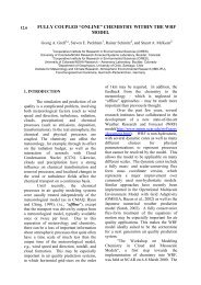
5.4 - IMPACT OF A SNOW PHYSICS PARAMETERIZATION ON SHORT-RANGE
FORECASTS OF SKIN TEMPERATURE IN MAPS/RUC
Tatiana G. Smirnova
Cooperative Institute for Research in Environmental Sciences (CIRES)
University of Colorado/NOAA Forecast Systems Laboratory
Boulder, Colorado
John M. Brown and Stanley G. Benjamin
NOAA Forecast Systems Laboratory
Boulder, Colorado
1. INTRODUCTION
A snow physics parameterization and snow cycling
component has been added to the soil/vegetation scheme
(Smirnova et al., 1997b) previously incorporated into the forecast
component of MAPS (Mesoscale Analysis and Prediction
System, Benjamin et al. 1996, 1997). (MAPS is implemented
at the National Centers for Environmental Prediction (NCEP)
as the Rapid Update Cycle or RUC.) The snow physics package
accounts for the processes of snow accumulation on the ground
surface and snow melting. Our goal here is to improve MAPS/
RUC prediction of skin temperature and surface air temperature,
and avoid the significant errors which may result even at
short time scales from inaccurate forecasts of snow cover. The
snow model, its testing in a 1-D framework, and implementation
in the 3-D forecast scheme are discussed in the paper.
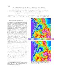
Figure.1 A summary of the processes in the MAPS/RUC
soil/snow/vegetation scheme.
2. SNOW MODEL DESCRIPTION
The MAPS/RUC soil model contains heat and moisture
transfer equations together with the energy and moisture budget
equations for the ground surface, and uses an implicit
scheme for the computation of the surface fluxes. The heat and
moisture budgets are applied to a thin layer spanning the
ground surface and including both the soil and the atmosphere
with corresponding heat capacities and densities (Fig. 1). A
concept for treating the evapotranspiration process, developed
by Pan and Mahrt (1987), is implemented in the MAPS/RUC
soil/vegetation scheme.
In the presence of snow cover, snow is considered to be
an additional upper layer of soil that interacts with the atmosphere,
significantly affecting its characteristics. The properties
of snow are quite different from those of soil. High values of albedo
reduce the amount of absorbed solar radiation, and the
small thermal diffusivity in snow reduces coupling with temperatures
in the soil layers below. As a result, the skin temperature
may be much cooler where there is snow cover. Further,
the atmospheric stratification frequently becomes stable with
inversions near the ground.
The snow model contains a heat-transfer equation within
the snow layer together with the energy and moisture budget
equations on the surface of the snow pack. This budget is applied
to the entire snow layer if snow depth is less than a threshold
value, currently set equal to 7.5 cm, or to the top 7.5 cm
layer of snow if the snow pack is thicker. Snow evaporates at a
potential rate unless the snow layer would all evaporate before
the end of the time step. In this case the evaporation rate is reduced
to that which would just evaporate all the existing snow
during the current time step. Heat flux within the snow layer is
calculated with a constant value of thermal conductivity of 0.25
Wm -1 K -1 , the average of values for new and old snow (Table
11-3, Pielke 1984). Averaged values from the same source are
used for specific heat capacity of snow (2090 J kg -1 K -1 ) and
snow density (290 kg m -3 ). A heat budget is also calculated at
Corresponding author address: Tatiana G. Smirnova, NOAA/
ERL/FSL, R/E/FS1, 325 Broadway, Boulder, CO 80303, e-
mail: smirnova@fsl.noaa.gov

the boundary between the snow pack and the soil, allowing
melting from the bottom of the snow layer. Melting at the top
or bottom of the snow layer occurs if energy budgets produce
temperatures higher than the freezing temperature (0 o C). In
this case the snow temperature is set equal to the freezing point,
and the residual from the energy budget is spent on melting
snow. Water from melting snow infiltrates into the soil, and if
the infiltration rate exceeds the maximum possible value for the
given soil type, then the excess water becomes surface runoff.
The accumulation of snow on the ground surface is provided
by the microphysics algorithm of the MAPS/RUC forecast
scheme (Reisner et al. 1997, Brown et al. 1998). It predicts
the total amount of precipitation and also the distribution of
precipitation between the solid and liquid phase. The subgridscale
(“convective”) parameterization scheme also contributes
to the liquid precipitation. With or without snow cover, the liquid
phase is infiltrated into the soil at a rate not exceeding maximum
infiltration rate, and the excess goes into surface runoff.
The solid phase in the form of snow or graupel is accumulated
on the ground/snow surface and is unavailable for the soil until
melting begins.
3. ONE-DIMENSIONAL EXPERIMENTS
The MAPS snow model was tested off-line in a one-dimensional
(1-D) setting before incorporation into the MAPS/
RUC forecast scheme. The data from six stations located in the
different climatic regions of the former Soviet Union, provided
by Adam Schlosser (pers. comm.) and described by Robock et
al. (1995), are excellent for such testing. In these 1-D experiments,
the model simulates moisture and heat transfers inside
the soil, and interaction processes between the ground/snow
surface and the atmosphere, including surface fluxes, snow accumulation,
and snow melting, driven by atmospheric forcing
for a six-year period (1978-1983). The datasets for all six stations
have a 3-hour frequency, and are interpolated to 30-
minute intervals. The first year of simulations is repeated until
an equilibrium state is reached, when the result is no longer dependent
on the initial conditions. The simulated surface temperature,
soil moisture, and snow water equivalent are verified
against the real data to evaluate the performance of the snowmelting
algorithm.
Figure 2 depicts various observed and simulated variables
over the 6-year period for Khabarovsk, located in a moist
forest area of Russia. The model captures the main features in
the seasonal variations of soil moisture and also demonstrates
consistency with precipitation events and periods of active
snow melting. The snow water equivalent also appears to be in
good agreement with observations. There are two main seasonal
spikes in the moisture available for infiltration into soil (Fig.
2a): the first is in spring when the snow is melting, and the second
is in the fall and is related to the precipitation maximum at
that time. The driest periods of the year are the end of summer
and winter. Similar features can be traced in the soil moisture
content of the top 1 m (Fig. 2b), where there is also generally
good agreement between the model and observations. The exception
is 1980, when observed soil moisture values in spring
and fall far exceeded both field capacity and model simulations.
The year 1980 also had an abnormally large seasonal variation
of observed soil moisture in comparison to the other five years.
We can only speculate that the uncertainty of determining soil
hydraulic properties in the model and the disregard of variation
with depth of soil properties such as porosity and density may
play an important role in this extreme situation, and yet provide
reasonable performance of the model in other situations.
.
1978 1979 1980 1981 1982 1983
1978 1979 1980 1981 1982 1983
1978 1979 1980 1981 1982 1983
Figure 2. MAPS 1-D model results and observations
from 1978-83 for Khabarovsk, Russia. a) Accumulation (mm)
of observed precipitation and simulated runoff and snow melt;
b) volumetric soil moisture in top 1 m of soil; and c) observed
and simulated snow water equivalent over 10-day periods.
a
b
c

The performance of the MAPS/RUC soil/snow/vegetation
scheme in dry climatic conditions is also tested. Data from
Uralsk, located in the semiarid continental area of Kazakhstan,
is appropriate for this purpose (Fig. 3 a,b,c). The small annual
precipitation at Uralsk usually has a minimum during the warm
season. The precipitation forcing in the 1-D experiments is the
water equivalent of observed precipitation, and the 1-D model
considers it to be snow if the atmospheric temperature is below
freezing. This assumption works better for the regions with
steady snow cover and low temperatures in winter. But, for
Uralsk with its significant temperature variations, snow which
in fact may fall at temperatures slightly above 0 o C might be incorrectly
designated as rain. This could explain the underestimation
of snow water equivalent (Fig. 3c). The snow melting
process at this location takes place during the entire cold season
(Fig. 3a), and not just in spring or early fall as at Khabarovsk
(Fig. 2a). The simulated moisture volume in the top1mofsoil
has spikes in the cold seasons corresponding to the spikes of
snow melt or precipitation (Fig. 3b). In most cases the response
is adequate, although in January 1979 and December 1980 it is
slightly overestimated. This behavior may be improved by taking
into account frozen soil physics, which reduces moisture infiltration
into frozen soil. In summertime, soil moisture content
drops to the wilting point level as happens in reality, but changes
corresponding to the summer precipitation events have less
amplitude than the observed soil moisture.
Experiments were also conducted for four other stations,
and overall the model demonstrated good performance of
its snow-accumulating and snow-melting algorithms both in
dry and wet climates. This off-line testing of the soil/snow/vegetation
scheme was the basis for its incorporation into the 40km
MAPS three-dimensional forecast scheme running in real time.
In April 1996, the multilevel soil/vegetation model was
introduced into the continuously running MAPS assimilation
system. The soil temperature and volumetric water content
fields, as predicted by the soil model, have been allowed to
evolve in the MAPS 3-hourly assimilation cycle over the 18
months (as of this writing) since that time. Because there is not
yet a high-frequency, national domain precipitation analysis
available in real time, it is necessary to depend on the MAPS 3-
hourly precipitation forecasts for precipitation input. A description
of the evolution of MAPS soil fields is presented by
Smirnova et al. (1997; also available on-line at http://
maps.fsl.noaa.gov/papers/smirnova/ams97_feb.newgif.html)
Since January 1997, a snow model with accumulation
and melting processes and a full energy budget has been running
in the real-time MAPS. This scheme was made possible
by the addition in the same month of a relatively sophisticated
cloud microphysics scheme (the level 4 scheme from the
NCAR/Penn State MM5 research model, Reisner et al. 1997,
Brown et al. 1998), allowing for the formation, transport and
fallout of cloud water and cloud ice as well as rain, snow, graupel,
and the number concentration of cloud ice particles. The
scheme assumes an exponential distribution of precipitation
particles and permits the coexistence at a grid point, if the temperature
is between 0 ° and -40 ° C, of both water and ice hydrometeors.
Along with the introduction of this scheme, a
hydrometeor cycling capability has been added to MAPS, so
that cloud fields from the previous 1-h forecast are used to initialize
each new forecast, minimizing cloud spin-up.
1978 1979 1980 1981 1982 1983
a
b
4. THREE-DIMENSIONAL APPLICATION
1978 1979 1980 1981 1982 1983
c
c
1978 1979 1980 1981 1982 1983
1978 1979 1980 1981 1982 1983
Figure 3. Same as Fig. 2 but for Uralsk, Kazakhstan.

From January through March 1997, the snow fields in
MAPS were allowed to cycle over each 24-h period, with an
update of the snow depth field occurring once daily from the
USAF snow cover analysis. That analysis was a large improvement
over using no snow cover at all, but has shown serious
problems in certain situations such as continuous low cloud
cover. Since early March 1997 through the end of May, the
USAF analysis has been unavailable and, consequently, the
snow cover field in MAPS has been allowed to cycle independently,
as have the soil moisture and temperature fields. The results
of this test (forced by external circumstances) have been
very satisfactory, and suggest that, even with an improved snow
analyses in the future, model forecast snow information should
be combined with observation-based analyses to determine optimal
snow fields.
Figures demonstrating the impact of snow physics parameterization
on the forecast of skin and surface air temperature
in the ongoing MAPS assimilation cycle will be presented
at the meeting.
5. CONCLUDING REMARKS
Off-line one-dimensional testing of our soil/snow/vegetation
scheme with snow accumulation and melting processes
and a full energy budget has been undertaken on the data from
several Russian stations. The model has demonstrated good
performance in capturing the main features in seasonal changes
of soil moisture and in the simulation of snow accumulation
and snow melting. Further improvement of its results may be
achieved by more accurate treatment of soil properties with the
possibility of changing these properties with depth, by defining
snow characteristics as a function of the snow age, and also by
the incorporation of frozen soil physics into the current version
of the scheme.
The soil/snow/vegetation model has a 9-month history
(as of this writing) since its implementation into the ongoing 3-
D MAPS cycle. Qualitative verification of soil moisture, snow
accumulation, and snow melt fields shows that these fields, in
general, are quite realistic. Further, low-level atmospheric temperature
forecasts are generally improved in regions of snow
cover, particularly in areas of recent snowfall or rapid melting.
Eleventh Conference on Numerical Weather Prediction,
Norfolk, VA, Amer. Meteor. Soc., 161-163.
Brown, J. M., T. G. Smirnova, and S, G, Benjamin, 1998:
Introduction of MM5 level 4 microphysics into the
RUC-2. Twelfth Conference on Numerical Weather
Prediction, Phoenix, AZ, Amer. Meteor. Soc., (Paper
4A.4).
Pan, H.-L. and L. Mahrt, 1987: Interaction between soil
hydrology and boundary-layer development. Bound.-
Layer Meteorol., 38, 185-202.
Pielke, R. A., 1984: Mesoscale meteorological modeling. Academic
Press, San Diego, CA, 612 pp.
Reisner, J., R. M. Rasmussen, and R.T. Bruintjes, 1997:
Explicit forecasting of supercooled liquid water in
winter storms using a mesoscale model. Quart. J. Roy.
Meteor. Soc., in press.
Robock, A., K. Ya. Vinnikov, and C. A. Schlosser, 1995: Use
of midlatitude soil moisture and meteorological observations
to validate soil moisture simulations with biosphere
and bucket models. J. of Climate, 8, 15-35.
Smirnova, T. G., J. M. Brown, and S. G. Benjamin, 1997a:
Evolution of soil moisture and temperature in the
MAPS/RUC assimilation cycle. 13th Conference on
Hydrology, Long Beach, CA, Amer. Meteor. Soc., 172-
175.
Smirnova, T. G., J. M. Brown, and S. G. Benjamin, 1997b:
Performance of different soil model configurations in
simulating ground surface temperature and surface
fluxes. Mon. Wea. Rev., 125, 1870-1884.
6. REFERENCES
Benjamin, S.G., J.M. Brown, K.J. Brundage, D. Devenyi, D.
Kim, B.E. Schwartz, T.G. Smirnova, T.L. Smith, and
A. Marroquin, 1997: Improvements in aviation forecasts
from the 40-km RUC. 7th Conference on Aviation,
Range, and Aerospace Meteorology, Long Beach,
CA, Amer. Meteor. Soc., 411-416.
Benjamin, S. G., J. M. Brown, K. J. Brundage, D. Devenyi, B.
Schwartz, T. G. Smirnova, T. L. Smith, and F.-J.Wang,
1996: The 40-km 40-level version of MAPS/RUC.