WRF/Chem Version 3.3 User's Guide - RUC - NOAA

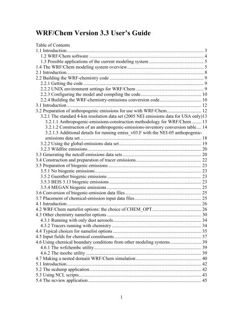
WRF/Chem Version 3.3 User’s GuideTable of Contents1.1 Introduction ................................................................................................................... 3 1.2 WRF/Chem software ................................................................................................ 4 1.3 Possible applications of the current modeling system .............................................. 5 1.4 The WRF/Chem modeling system overview ................................................................ 5 2.1 Introduction ................................................................................................................... 8 2.2 Building the WRF-chemistry code ............................................................................... 9 2.2.1 Getting the code ..................................................................................................... 9 2.2.2 UNIX environment settings for WRF/Chem ......................................................... 9 2.2.3 Configuring the model and compiling the code ................................................... 10 2.2.4 Building the WRF-chemistry-emissions conversion code ................................... 10 3.1 Introduction ................................................................................................................. 12 3.2 Preparation of anthropogenic emissions for use with WRF/Chem ............................. 12 3.2.1 The standard 4-km resolution data set (2005 NEI emissions data for USA only)13 3.2.1.1 Anthropogenic-emissions-construction methodology for WRF/Chem ........ 13 3.2.1.2 Construction of an anthropogenic-emissions-inventory conversion table .... 14 3.2.1.3 Additional details for running emiss_v03.F with the NEI-05 anthopogenicemissionsdata set ...................................................................................................... 18 3.2.2 Using the global-emissions data set ..................................................................... 19 3.2.3 Wildfire emissions ............................................................................................... 20 3.3 Generating the netcdf-emissions data sets .................................................................. 20 3.4 Construction and preparation of tracer emissions ....................................................... 22 3.5 Preparation of biogenic emissions .............................................................................. 23 3.5.1 No biogenic emissions ......................................................................................... 23 3.5.2 Guenther biogenic emissions ............................................................................... 23 3.5.3 BEIS 3.13 biogenic emissions ............................................................................. 23 3.5.4 MEGAN biogenic emissions ............................................................................... 25 3.6 Conversion of biogenic-emission data files ................................................................ 25 3.7 Placement of chemical-emission input data files ........................................................ 25 4.1 Introduction ................................................................................................................. 26 4.2 WRF/Chem namelist options: the choice of CHEM_OPT ......................................... 26 4.3 Other chemistry namelist options ............................................................................... 30 4.3.1 Running with only dust aerosols .......................................................................... 34 4.3.2 Tracers running with chemistry ........................................................................... 34 4.4 Typical choices for namelist options .......................................................................... 35 4.5 Input fields for chemical constituents ......................................................................... 37 4.6 Using chemical boundary conditions from other modeling systems .......................... 39 4.6.1 The wrfchembc utility .......................................................................................... 39 4.6.2 The mozbc utility ................................................................................................. 39 4.7 Making a nested domain WRF/Chem simulation ....................................................... 40 5.1 Introduction ................................................................................................................. 42 5.2 The ncdump application .............................................................................................. 42 5.3 Using NCL scripts....................................................................................................... 43 5.4 The ncview application ............................................................................................... 45 1

5.5 The RIP application .................................................................................................... 46 5.5.1 Downloading and installing the RIP program ..................................................... 46 5.5.2 Pre-processing data from WRF/Chem ................................................................. 47 5.5.3 Generating NCAR GKS plots using RIP ............................................................. 48 6.1 Introduction ................................................................................................................. 51 6.2 KPP requirements ....................................................................................................... 52 6.3 Compiling the WKC ................................................................................................... 52 6.4 Implementing chemical mechanisms with WKC ....................................................... 52 6.5 Layout of WKC ........................................................................................................... 53 6.6 Code produced by WKC, User Modifications ............................................................ 54 6.7 Available integrators ................................................................................................... 55 6.8 Adding mechanisms with WKC ................................................................................. 55 6.9 Adapting KPP equation files ....................................................................................... 56 6.10 Adapting additional KPP integrators for WKC ........................................................ 57 7.1 Summary ..................................................................................................................... 58 7.2 WRF/Chem publications ............................................................................................. 58 Appendix A : WRF/Chem Quick Start Guide .................................................................. 66 Appendix B : Using prep_chem_sources V1 .................................................................... 73 Appendix C: Using prep_chem_sources V1.1.1 ............................................................... 85 Appendix D: Using MEGAN with WRF/Chem ............................................................... 88 Appendix E: Using MOZART with WRF/Chem ............................................................. 91 Appendix F: Using the Lightning-NOx Parameterization ................................................ 93 2

WRF/Chem Version 3.3 User’s GuideWRF/Chem OverviewTable of Contents1.1 Introduction ................................................................................................................... 31.2 WRF/Chem software .................................................................................................... 41.3 Possible applications of the current modeling system .................................................. 51.4 The WRF/Chem modeling system overview ................................................................ 51.1 IntroductionThe WRF/Chem User’s Guide is designed to provide the reader with informationspecific to the chemistry part of the WRF model and its potential applications. It willprovide the user a description of the WRF/Chem model and discuss specific issuesrelated to generating a forecast that includes chemical constituents beyond what istypically used by today’s meteorological forecast models. For additional informationregarding the WRF model, the reader is referred to the WRF model User’s Guide(http://www.mmm.ucar.edu/wrf/users/docs/user_guide_V33/contents.html).Presently, the WRF/Chem model is now released as part of the Weather Researchand Forecasting (WRF) modeling package. And due to this dependence upon WRF, it isassumed that anyone choosing to use WRF/Chem is very familiar with the set-up and useof the basic WRF model. It would be best for new WRF users to first gain training andexperience in editing, compiling, configuring, and using WRF before venturing into themore advanced realm of setting up and running the WRF/Chem model.The WRF/Chem model package consists of the following components (in additionto resolved and non-resolved transport):§ Dry deposition, coupled with the soil/vegetation scheme§ Four choices for biogenic emissions: No biogenic emissions included Online calculation of biogenic emissions as in Simpson et al. (1995) and Guentheret al. (1994) includes emissions of isoprene, monoterpenes, and nitrogenemissions by soil Online modification of user-specified biogenic emissions - such as the EPABiogenic Emissions Inventory System (BEIS) version 3.13. The user mustprovide the emissions data for their own domain in the proper WRF data fileformat Online calculation of biogenic emissions from MEGAN§ Three choices for anthropogenic emissions: No anthropogenic emissions3

User-specified anthropogenic emissions such as those available from the EPANEI-05 data inventory. The user must provide the emissions data for their owndomain in the proper WRF data file format Global emissions data from the one-half degree RETRO and ten-degree EDGARdata sets§ Several choices for gas-phase chemical mechanisms including: RADM2, RACM, CB-4 and CBM-Z chemical mechanisms The use of the Kinetic Pre-Processor, (KPP) to generate the chemicalmechanisms. The equation files (using Rosenbrock type solvers) are currentlyavailable for RADM2, RACM, RACM-MIM, SAPRC-99, MOZART chemicalmechanisms as well as others§ Three choices for photolysis schemes: Madronich scheme coupled with hydrometeors, aerosols, and convectiveparameterizations. This is a computationally intensive choice, tested with manysetups Fast-J photolysis scheme coupled with hydrometeors, aerosols, and convectiveparameterizations F-TUV photolysis scheme. This scheme, also from Sasha Madronich is faster, butdoes not work with all aerosol options§ Three choices for aerosol schemes: The Modal Aerosol Dynamics Model for Europe - MADE/SORGAM The Model for Simulating Aerosol Interactions and Chemistry (MOSAIC - 4 or 8bins) sectional model aerosol parameterization A total mass aerosol module from GOCART§ Aerosol direct effect through interaction with atmospheric radiation, photolysis, andmicrophysics routines. In version 3.3 this is available for GOCART, MOSAIC orMADE/SORGAM options§ Aerosol indirect effect through interaction with atmospheric radiation, photolysis, andmicrophysics routines. In V3.3 this option is available for MOSAIC orMADE/SORGAM§ A tracer transport option in which the chemical mechanism, deposition, etc. has beenturned off. The user must provide the emissions data for their own domain in theproper WRF data file format for this option. May be run parallel with chemistry§ A plume rise model to treat the emissions of wildfires1.2 WRF/Chem softwareThe chemistry model has been built to be consistent with the WRF model I/OApplications Program Interface (I/O API). That is, the chemistry model section has beenbuilt following the construction methodology used in the remainder of the WRF model.Therefore, the reader is referred to the WRF software description in the WRF User’sGuide (Chapter 7) for additional information regarding software features like the buildmechanism and adding arrays to the WRF registry.4

1.3 Possible applications of the current modeling system§§§§Prediction and simulation of weather, or regional and local climateCoupled weather prediction/dispersion model to simulate release and transport ofconstituentsCoupled weather/dispersion/air quality model with full interaction of chemicalspecies with prediction of O 3 and UV radiation as well as particulate matter (PM)Study of processes that are important for global climate change issues. Theseinclude, but are not restricted to the aerosol direct and indirect forcing1.4 The WRF/Chem modeling system overviewThe following figure shows the flowchart for the WRF/Chem modeling system version3.3.5

As shown in the diagram, the WRF/Chem modeling system follows the same structure asthe WRF model by consisting of these major programs:§The WRF Pre-Processing System (WPS)6

§§§WRF-Var data assimilation systemWRF solver (ARW, o r NMM core) including chemistryPost-processing and visualization tools7

Chapter 2: WRF/Chem Software InstallationTable of Contents2.1 Introduction ................................................................................................................... 82.2 Building the WRF-chemistry code ............................................................................... 92.2.1 Getting the code ..................................................................................................... 92.2.2 UNIX environment settings for WRF/Chem ......................................................... 92.2.3 Configuring the model and compiling the code ................................................... 102.2.4 Building the WRF-chemistry emissions conversion code ................................... 102.1 IntroductionThe WRF modeling system software (including chemistry) installation isstraightforward on the ported platforms. The package is mostly self-contained, meaningthat WRF requires no external libraries that are not already supplied with the code. Oneexception is the netCDF library, which is one of the supported I/O API packages. ThenetCDF libraries or source code are available from the Unidata homepage athttp://www.unidata.ucar.edu (select DOWNLOADS, registration required, to find thenetCDF link).The WRF/Chem model has been successfully ported to a number of Unix-basedmachines. We do not have access to all tested systems and must rely on outside users andvendors to supply required configuration information for compiler and loader options ofcomputing architectures that are not available to us. See also chapter 2 of the User’sGuide for the Advanced Research WRF for a list of the supported combinations ofhardware and software, required compilers, and scripting languages as well as postprocessingsoftware. It cannot be guaranteed that chemistry will build successfully on allarchitectures that have been tested for the meteorological version of WRF.Note that this document assumes a priori that the reader is very familiar with theinstallation and implementation of the WRF model and its initialization package (e.g., theWRF Standard Initialization program, or WPS). Documentation for the WRF Model andits initialization package can be found at (http://www.mmm.ucar.edu/wrf/users/pubdoc.html).With this assumption in place, the remainder of this chapter provides a quickoverview of the methodology for downloading the WRF/Chem code, setting the requiredenvironmental variables, and compiling the WRF/Chem model. Subsequent chaptersassume that the user has access to the WRF/Chem model- and emission-data sets for theirregion of interest and has them readily available so that a full weather and chemicaltransport simulation can be conducted.8

2.2 Building the WRF-chemistry code2.2.1 Getting the code§§Download, or copy to your working space, the WRF zipped tar file.• The WRF model and the chemistry code directory are available from theWRF model download web site (http://www.mmm.ucar.edu/wrf/users)• The chemistry code is a separate download from the WRF modeldownload web page and can be found under the WRF-Chemistry code title• Always get the latest version if you are not trying to continue a longproject• Check for known bug fixes for both, WRF and WRF-ChemUnzip and untar the file• > gzip –cd WRFV3-Chem-3.3.TAR | tar –xf –• Again, if there is a newer version of the code use it, 3.3 is used only as anexample• > cd WRFV3Remember that bug fixes become available on a regular basis and can be downloadedfrom the WRF/Chem web site (http://www.wrf-model.org/WG11). You should check thisweb page frequently for updates on bug fixes. This includes also updates and bug fixesfor the meteorological WRF code (http://www.mmm.ucar.edu/wrf/users/).2.2.2 UNIX environment settings for WRF/ChemBefore building the WRF/Chem code, several environmental settings are used tospecify whether certain portions of the code need to be included in the model build. In c-shell syntax, the important environmental settings are:setenv WRF_EM_CORE 1setenv WRF_NMM_CORE 0and they explicitly define which model core to build. These are the default values that aregenerally not required. The environmental settingsetenv WRF_CHEM 1explicitly defines that the chemistry code is to be included in the WRF model build, andis required for WRF/Chem. This variable is required at configure time as well as compiletime.Optionally,setenv WRF_KPP 19

setenv YACC ‘/usr/bin/yacc –d’setenv FLEX_LIB_DIR /usr/local/libexplicitly defines that the Kinetic Pre-Processor (KPP) (Damian et al. 2002; Sandu et al.2003; Sandu and Sander 2006) is to be included in the WRF/Chem model build using theflex library (libfl.a). In our case, the flex library is located in /usr/local/lib and compilesthe KPP code using the yacc (yet another compiler compiler) location in /usr/bin. This isoptional as not all chemical mechanisms need the KPP libraries built during compilation.The user may first determine whether the KPP libraries will be needed (see chapter 6 fora description of available options). One should set the KPP environmental variable tozero (setenv WRF_KPP 0) if the KPP libraries are not needed.2.2.3 Configuring the model and compiling the codeThe WRF code has a fairly complicated build mechanism. It tries to determine thearchitecture that you are on, and then present you with options to allow you to select thepreferred build method. For example, if you are on a Linux machine, the code mechanismdetermines whether this is a 32-or 64-bit machine, and then prompts you for the desiredusage of processors (such as serial, shared memory, or distributed memory) andcompilers. Start by selecting the build method:§§§§> ./configureChoose one of the options• Usually, option "1" is for a serial build. For WRF/Chem. Do not use theshared memory OPENMP option (smpar, or dm + sm), these are notsupported. The serial build is a preferred choice if you are debugging theprogram and are working with very small data sets (e.g. if you aredeveloping the code). Since WRF/Chem uses a lot of memory (manyadditional variables), the distributed memory options are preferred for allother casesYou can now compile the code using• > ./compile em_real >& compile.logIf your compilation was successful, you should find the executables in the“main” subdirectory. You should see ndown.exe, real.exe, and wrf.exe listed• > ls -ls main/*.exe2.2.4 Building the WRF-chemistry-emissions-conversion codeAfter building the WRF-Chemistry model, you can then compile the conversionprograms that will allow you to run the anthropogenic- and biogenic-emissions programs.These programs are used to convert “raw” anthropogenic-and biogenic-data files intoWRF netCDF input data files. In the WRFV3 directory, type the following commands:10

§§§> ./compile emi_conv> ls -ls WRFV3/chem/*.exe• You should see the file convert_emiss.exe listed in the chemistrydirectory. This file should already be linked to the WRFV3/test/em_realdirectory.> ls -ls WRFV3/test/em_real/*.exe• You should see the files ndown.exe, real.exe, wrf.exe, convert_emiss.exe,listed in the em_real directory.11

Chapter 3: Generation of WRF/Chem-Emissions DataTable of Contents3.1 Introduction .............................................................................................................. 12 3.2 Preparation of anthropogenic emissions for use with WRF/Chem ............................. 12 3.2.1 The standard 4-km resolution data set (2005 NEI emissions data for USA only)13 3.2.1.1 Anthropogenic-emissions construction methodology for WRF/Chem ......... 13 3.2.1.2 Construction of an anthropogenic-emissions-inventory conversion table .... 14 3.2.1.3 Additional details for running emiss_v03.F with the NEI-05 anthopogenicemissionsdata set ...................................................................................................... 18 3.2.2 Using the global-emissions data set ..................................................................... 19 3.2.3 Wildfire emissions ............................................................................................... 20 3.3 Generating the netcdfemissions data sets ................................................................... 20 3.4 Construction and preparation of tracer emissions ....................................................... 22 3.5 Preparation of biogenic emissions .............................................................................. 23 3.5.1 No biogenic emissions ......................................................................................... 23 3.5.2 Guenther biogenic emissions ............................................................................... 23 3.5.3 BEIS 3.13 biogenic emissions ............................................................................. 23 3.5.4 MEGAN biogenic emissions ............................................................................... 25 3.6 Conversion of biogenic-emission data files ................................................................ 25 3.7 Placement of chemical-emission input data files ........................................................ 25 3.1 IntroductionOne of the main differences between running with and without chemistry is theinclusion of additional data sets describing the sources of chemical species. At this time,these files need to be prepared externally from the WRF/Chem simulation due to the widevariety of data sources. This places the WRF/Chem user in a position of needing tounderstand the complexity of their emissions data as well as having the control over howthe chemicals are speciated and mapped to their simulation domain. While this can be adaunting task to the uninitiated, the following section will illustrate the methodologythrough which emissions data is generated for a forecast domain.3.2 Preparation of anthropogenic emissions for use with WRF/ChemAt this time there is no single tool that will construct an anthropogenic- emissionsdata set for any domain and any chemical mechanism that you select. This places therequirement upon you to construct the anthropogenic-emissions data set for yourparticular domain and desired chemistry. However, several programs and data sets areprovided that you may use to create an emissions data set, if your domain and yourchoice of chemical mechanism follow some restrictions. These programs are described in12

the following two subsections. Note that you must know a priori the preferred domainlocation and chemistry options that will be used in the simulation. The "raw"anthropogenic-emissions data set described next can be used if the domain is located overthe 48 contiguous states of the United States. The next section shows the suggestedmethodology for constructing your own anthropogenic-emissions data set.3.2.1 The standard 4-km resolution data set (2005 NEI emissions data for USA only)Anthropogenic-emissions data is currently available for the contiguous 48 statesof the United States, southern Canada and northern Mexico based upon the U.S.Environmental Protection Agency (EPA) National Emissions Inventory (NEI) 2005inventory. Area type emissions are available on a structured 4-km grid, while point typeemissions are available by latitude and longitude locations and with stack parametersneeded for plume-rise calculations. This data is discussed later in this section and can befound online at http://ruc.noaa.gov/wrf/WG11/anthropogenic.htm. For those who desireto conduct simulations over other regions of the world, the reader is referred to thesection in the appendix that describes the use of a global anthropogenic-emissionsinventory for the WRF/Chem model. The methodology for transferring ananthropogenic-emissions data set to the WRF model is discussed in the following section.3.2.1.1 Anthropogenic-emissions construction methodology for WRF/ChemThe methodology for constructing your own anthropogenic-emissions data set is:§§§§Obtain the “raw” anthropogenic-emissions data. This data could come from avariety of data sources and be on multiple map projections and/or domains.o A 4-km emissions data set (area) and point source is available for the U.S.(see below). Use of this data is recommended when the simulationdomain has a horizontal grid spacing of 12 km or greater.Specify, or make a table listing that relates “raw” emissions to the speciation ofthe desired chemical mechanism and PM mechanism (see following section)o The provided routines (emiss_v03.F) assume that the RADM2 chemicalmechanism and MADE/SORGAM modal aerosol models are being usedin the simulation.Prepare the 3-D (or 2-D) anthropogenic-emissions data seto Account for rise of emissions from stack, biomass burning, etc.o Output data in an intermediate format (binary for the U.S. NEI05 case).You can change format to match your needs inmodule_input_chem_data.FConvert the emissions data to a WRF netCDF data fileo Convert intermediate format (binary) emissions to 4-D WRF netcdf files(with executable of convert_emiss.F subroutine)o Input data format must match that used in the conversion routine (seemodule_input_chem_data.F)o Map data (extracted from the header in file wrfinput_d01) is needed forsome plotting routines to function properly.13

§If running WRF/Chem with a carbon bond type mechanism (CBM4, CBMZ, etc.),be sure to use the correct emiss_inpt_opt setting for the chemical mechanism.The WRF/Chem code will assume the emissions are in RADM2 form and willrepartition the emitted species to the appropriate carbon bond mechanism unlessyou specify a different choice with the emiss_inpt_opt. In addition, theSORGAM emissions will be converted to the 4- or 8- size bins for use in theMOSAIC aerosol routines.3.2.1.2 Construction of an anthropogenic-emissions-inventory conversion tableBegin with a list of known chemical species that are emitted in the domain of interest.These species may need to be translated into a list of chemical species that are used byyour particular photochemical and aerosol mechanisms within the WRF-Chemistrymodel. If you are uncertain about the names and units of the emissions data, theregistry.chem file in the WRFV3/Registry subdirectory contains the names anddimensions of the chemical species used within the WRF/Chem model.The translation from “raw” to WRF/Chem species emissions will often result in eitherlumping several emitted chemical species into one simulated species, or the partitioningof one emitted species into fractions of several simulated species. As an example, thefollowing emission assignment table (Table. 3.2) translates the “raw” NEI05 basedemission species into the WRF/Chem RADM2 species. The columns contain thefollowing information:§§§§§names of the emitted species in the “raw” data derived from the EPA NEI05inventory, VOC speciation is that used in the SAPRC-99 chemical mechanism.names of the emitted species used in the WRF-Chemistry model, Variable names(e.g. e_co) must match the WRF/Chem Registry names of the emission variables.the fractional amount of the “raw” emitted species assigned to the model emissionname,the molecular weight (used as a switch in emiss_v03.F – applies only to primaryNOx, SO 2 , CO and NH 3 emissions),the technical name of the “raw” emitted speciesTable 3.2. Conversion table within emiss_v03.F used to produce input-emissionsdata for a WRF-chemistry simulation. This table lists the “raw” emission name, theemissions field name used in the WRF model, the weight factor applied to thechemical field, the molecular weight of the species (NOx, SO 2 , CO and NH 3 only)and the full species name. The fields are then converted to an emissions speciationsuitable for use with the RADM2 chemical mechanism (+MADE/SORGAM aerosolmodule).“raw” WRF/Chm Weight MW Species namename nameCO e_co 1.00 28 Carbon monoxideNOX e_no 1.00 46 Nitrogen Oxides (NO or NO 2 )14

SO2 e_so2 1.00 64 Sulfur dioxideNH3 e_nh3 1.00 17 AmmoniaHC02 e_eth 1.00 00 Alkanes with kOH

modePM02 e_so4i 0.20 01 Sulfate PM2.5 - nuclei modePM02 e_so4j 0.80 01 Sulfate PM2.5 - accumulation modePM03 e_no3i 0.20 01 Nitrate PM2.5 - nuclei modePM03 e_noj 0.80 01 Nitrate PM2.5 - accumulation modePM04 e_orgi 0.20 01 Organic PM2.5 - nuclei modePM04 e_orgj 0.80 01 Organic PM2.5 - accumulation modePM05 e_eci 0.20 01 Elemental Carbon PM2.5 - nuclei modePM05 e_ecj 0.80 01 Elemental Carbon PM2.5 - accumulation modePM10-PRIe_pm10 1.00 01 Unspeciated Primary PM10The next step is to construct a program that reads the “raw” anthropogenic-emissionsdata, converts each chemical species to those used by the WRF/Chem model followingthe information from your particular conversion table and finally maps it onto the 3-dimensional simulation domain. Therefore, within this step any plume rise, or abovesurface anthropogenic emission placement needs to be specified. Particular attention togeospatial details, such as the WRF/Chem domain grid locations, and the elevation ofmodel vertical levels relative to the “raw ” emissions data set must be considered.Provided on the WRF/Chem ftp site is a program that can be used with the NEI-05U.S. anthropogenic-emissions inventory - emiss_v03.F. While your application may notuse the “raw” emissions data for your simulation, it is provided as an example of theadopted methodology. The product of the program is a binary data file containing threedimensionalemissions data, output at each hour that is mapped to a specified simulationdomain. The data format in the provided program is provided in Table 3.2.Table 3.2. Converted or “intermediate binary” emission data used to produceinput emissions data for a WRF-chemistry simulation. This table lists each outputvariable, its variable declaration, dimensions, and any additional information. Theoutput-data fields are specific to the RADM2 -chemical mechanism(+MADE/SORGAM aerosol module).File Declaration Dimensions Commentsvariablenv integer 1 Number of chemical speciesename character*9 30 Name of each emissions field in modelhour integer 1 Hour of the emissions data (begin loop)so2 real (nx,nz,ny)no real (nx,nz,ny)ald real (nx,nz,ny)hcho real (nx,nz,ny)ora2 real (nx,nz,ny)nh3 real (nx,nz,ny)hc3 real (nx,nz,ny)16

hc5 real (nx,nz,ny)hc8 real (nx,nz,ny)eth real (nx,nz,ny)ora2 real (nx,nz,ny)nh3 real (nx,nz,ny)co real (nx,nz,ny)ol2 real (nx,nz,ny)olt real (nx,nz,ny)oli real (nx,nz,ny)tol real (nx,nz,ny)xyl real (nx,nz,ny)ket real (nx,nz,ny)csl real (nx,nz,ny)iso real (nx,nz,ny)pm2.5i real (nx,nz,ny)pm2.5j real (nx,nz,ny)so4i real (nx,nz,ny)so4j real (nx,nz,ny)no3i real (nx,nz,ny)no3j real (nx,nz,ny)orgi real (nx,nz,ny)orgj real (nx,nz,ny)eci real (nx,nz,ny)ecj real (nx,nz,ny)pm10 real (nx,nz,ny) (end loop)For spatial partitioning, the emiss_v03.F program implicitly assumes the WRF/Chem gridhas a horizontal grid resolution larger than 4 km, and simple grid dumping from the“raw” 4-km domain into the specified WRF/Chem domain is appropriate. Currently noplume rise calculations directly couple WRF dynamics to anthropogenic point emissions.The emiss_v03.F routine includes some plume rise from the Brigg’s formulation due tomomentum lift from direct injection, and a specified horizontal wind climatology.Emissions within nested domains are also handled within emiss_v03.F by specifyingmother domain map parameters, the nested domain grid resolution, and beginning x and ylocations of the nested domain within the mother domain. These variable names arelisted, and described further in the following section.We assume that the anthropogenic-emissions data is updated at an hourly interval.However, the update interval is arbitrary and can be specified by you for your individualapplication. In addition, if the given binary format of the output data from emiss_v03.F isnot functional for your needs, the data format can be modified within the program.However, if the output data format is changed, the WRF/Chem program convert_emiss.Fwill also need to be modified so that the converted raw-emissions data can be read intothe program correctly and converted.17

Both surface and elevated point source emissions of gas-phase species are in units ofmole per square kilometer per hour, and in microgram per square meter per second(microgram m -2 s -1 ) for the aerosol species. These are the units assumed within theWRF/Chem input processor for the emissions files, and the convert_emiss.F processingstep that generates the netcdf emission file(s) described further below. (Conversion ofgas-phase emissions into the mixing ratio increases at each grid is handled withinmodule_emissions_anthropogenic.F . Aerosol increases due to emissions are handled inindividual aerosol mechanism modules.)It is entirely incumbent upon the user to specify location and time of emissions from the“raw” emissions for their own applications within this intermediate step of the emissionsprocessing.3.2.1.3 Additional details for running emiss_v03.F with the NEI-05 anthopogenicemissionsdata setThe “raw” anthropogenic-emissions data for the 48 contiguous states as well as selectregions of Canada and Mexico have been made available for download by theNOAA/Earth Systems Research Laboratory, Chemical Sciences Division. The process tocreate anthropogenic-emissions-input data files from this data is as follows:§§§§Before generation of the anthropogenic-emissions data file can begin, the real.exeprogram should be used to create the wrfinput_d01 and wrfbdy_d01 data files foryour desired domain. There are two reasons for doing this. The first is so that youknow exactly where the simulation domain is located. The second is because theemissions conversion program (convert_emiss.exe) will read the netCDF headerinformation from the wrfinput_d01 data file and write this information into the WRFchemical-emissionsdata files. If the wrfinput_d01 data file does not exist, theprogram will abort with an error.Download the raw-emissions data tar file from the anonymous ftp server(ftp://aftp.fsl.noaa.gov/divisions/taq/emissions_data_2005/em05v2_file*.tar) andextract the data into its own directory (e.g., $home/emissions_data).Download the emiss_v03.F program from the anonymous ftp server.Modify emiss_v03.F to set map and grid parameters for your particular domain aswell as the directory that contains the “raw” emissions data. For the provided testdomain you should have the following settings:Model variable Value DescriptionIl 40 east-west grid spacing (ix2+1) of mother domain andwest_east_stag dimension on your WRF domainJl 40 north-south grid spacing (jx2+1) of mother domain andsouth_north_stag dimension on your WRF domainIx2 39 x-dimension of user domain output data (IL-1)Jx2 39 y-dimension of user domain output data (JL-1)Kx 19 z-dimension of user domain output data or kemit on your WRF18

domain. The vertical dimension can equal or be less than that usedin the WRF domain.Inest1 0 nesting or no nesting flag (no nesting => inest1 = 0)Dx 60.E3 horizontal grid spacing (m) of user domainDxbigdo 60.E3 Horizontal grid spacing on mother domain (m)Xlatc 38.00 grid center latitude of mother domainXlonc -80.00 grid center longitude of mother domainClat1 38.001 Northern most reference latitude of projection (mother domain)Clat2 38.000 Southern most reference latitude of projection (CLAT1 > CLAT2for Lambert Conformal, CLAT2 not used for polar stereographic)Iproj 1 projection type (see WRFSI information)Rekm 6370. Earth radius (km)XNESSTR 1. x-location in mother domain of southwest corner point of the (1,1)grid in the user domain. Not used if Inest1=0 .YNESSTR 1. y-location in mother domain of southwest corner point of the (1,1)grid in the user domain. Not used if Inest1=0 .Datadir /data Path to directory holding emissions input data (character string)Zfa(See Elevation (m) at the top of each computational cellbelow)KWIN 20 Number of vertical levels in the horizontal wind profileWSPWind speed at level height(m) specified by REFWZREFWZElevation (m) of the specified horizontal wind profileDATA ZFA/ 0., 255., 515., 781., 1054., 1335., &1527., 1824., 2130., 2553., 2994., 3454., &4059., 4967., 6741., 8723.,10992.,14084., &16461.,20346./Note: the model ZFA height levels have been determined separately by processingthe wrfinput_d01 file generated by real.exe to add the vertical domain levels inmeters.§ Compile emiss_v03.F (single processor mode) with the command “pgf90 –Mfree –byteswapio –o emiss_v03.exe emiss_v03.F” and run emiss_v03exe. This program,using raw-emissions data, maps the emissions data to your specified domain andgenerates binary-emissions data files (file names are set in emiss_v03.F to bewrfem_00to12Z and wrfem_12to24Z).3.2.2 Using the global-emissions data setThe use of a global-missions data set has recently been added to WRF/Chemoptions. The global emissions data comes from the REanalysis of the TROpospheric(RETRO) chemical composition over the past 40 years (http://retro.enes.org/index.shtml)and Emission Database for Global Atmospheric Research (EDGAR)(http://www.mnp.nl/edgar/introduction). Both RETRO and EDGAR provide globalannual emissions for several greenhouse gases (e.g., CO2, CH4 and N2O) as well assome precursor gases on a .5x.5 degree (RETRO) or a 1x1 degree (EDGAR) grid.A simple grid-mapping program has been made available to WRF/Chem users.This program, called prep_chem_sources, was developed at CPTEC, Brazil and is19

available to WRF/Chem users. The program will map the global anthropogenicemissionsdata to a WRF-forecast domain using a polar stereographic or Lambertconformal projection. See appendix (B) for more information regarding theprep_chem_sources routine.3.2.3 Wildfire emissionsThe prep_chem_sources program (see appendix B) is capable of providingbiomass burning, or wildfire, emissions to the WRF/Chem forecast. The geostationaryNOAA weather satellite (GOES) provides half-hourly fire data for the WesternHemisphere. Specifically, GOES-12 provides coverage for North and South Americawhile GOES-11 covers North America only. Data files containing the WFABBA firelocation are distributed by the University of Wisconsin-Madison(http://cimss.ssec.wisc.edu/goes/burn/wfabba.html). The archived WF-ABBA data areavailable at this time from two different web sites; http://www.firedetect.noaa.gov andhttp://www.nrlmry.navy.mil.flambe/index.html. Additional wildfire location data isavailable from MODIS at the University of Maryland web site:http://firefly.geog.umd.edu/firms. The prep_chem_sources reads this data, the WFABBAdata files all being in one directory and MODIS from the same or different directory, andmaps the point source data to the WRF domain. It is also not too difficult to include othersources for wildfire emissions.In the WRF/Chem model, the wildfire-emissions data is obtained from thewrffirechemi_d01 emissions data file. It computes the plume rise of the wildfire smokebased upon the environmental wind and temperature profile. The emissions to theforecast are then provided as a vertical distribution based upon the results from the plumerise calculation.3.3 Generating the netcdf-emissions data setsThe final step in the process is to produce a WRF/Chem netCDF-emissions inputdata file containing all of the required metadata (map projection data, simulation starttime, etc.) for the simulation. Ideally the metadata contained in the WRF/Chem-emissionsfile would be generated by the previous step. However, if not provided by the user, theWRF input data file (e.g., wrfinput_d01) can be read and the metdata information addedto the anthropogenic-emissions input data file. The name of the final netcdf data file(s)can be either wrfchemi__d or wrfchemi_d_depending upon your intent (io_style_emissions option in namelist). The latter intent isdesigned for daily varying emissions (io_style_emissions=2), and in this case thedate/time specified in the WRF/Chem-emissions data file must match the simulationdate/time or no emissions data will be read and a run-time error will result. The firstintent (io_style_emissions=1) assumes you are creating two netcdf 4-D emission filesnamed wrfchemi_00z_d and wrfchemi_12z_ d that containhourly emissions from 00:00 to 11:00 UTC, and 12:00 to 23:00 UTC, respectively. Thisis the format generated by convert_emiss.F that matches the provided NEI-05 inventory.20

The NEI-05 inventory is representative of a “typical ozone season day” by the U.S. EPA,and is typically used for all days within multiday WRF/Chem simulations.§Before the conversion from “binary intermediate” to netcdf file emissions can begin,you need to change the namelist.input file in the WRFV3/test/em_real directory to theemissions data file settings. The settings that will generate 24 hours of hourlyemissions(i.e., io_style_emissions=2) data are:&time_controlrun_days = 1,run_hours = 0,run_minutes = 0,run_seconds = 0,start_year = 2008,start_month = 07,start_day = 14,start_hour = 00,start_minute = 00,start_second = 00,end_year = 2008,end_month = 07,end_day = 15,end_hour = 12,end_minute = 00,end_second = 00,auxinput6_inname = ‘wrfbiochemi_d,auxinput7_inname = ‘wrffirechemi_d,auxinput8_inname = ‘wrfchemi_gocart_bg_d,auxinput5_interval_m = 60,auxinput7_interval_m = 1440,auxinput8_interval_m = 1440,io_form_auxinput2 = 2,io_form_auxinput5 = 2,io_form_auxinput6 = 2,io_form_auxinput7 = 2,io_form_auxinput8 = 2,io_form_auxinput12 = 0,&chemchem_opt = 1,emiss_opt = 3,chem_in_opt = 0,bio_emiss_opt = 1.Starting with version 3.3, you should note that the name list setting for theauxiliary input port time interval is now dependent upon each input stream.That is, for the emissions conversion program convert_emiss.exe, the settings for21

each auxiliary input port specifies whether it is turned on, the IO format, the timeinterval for the emissions data updates and the number of frames in each file (notshown).§§§We assume that you have already configured and compiled the WRF/Chem model.So now build the emissions conversion program with the command “compileemi_conv” in WRFV3 directory.Run convert_emiss.exe for 24 hours starting at 0000 UTC and ending at 0000 UTCand save the netCDF wrfchemi_d01 data file aswrfchemi_d01_2008-07-14_00:00:00. The filename(s) need to match the name of theinput data file in mediation_integrate.F (see convert_emiss.F program inside theWRFV3/chem directory). The file(s) should be transferred (or linked) to yourWRFV3/test/em_real directory.Once the “wrfchemi” files are generated, it is best to plot fields or use a program likencview to examine the files that have been generated. Look at the files and confirmthat the emissions appear to match the WRF forecast domain you previouslygenerated. When looking at anthropogenic emissions (e.g., co) the surface emissionsshould look similar to a map with cities and possibly roads showing. Be sure toconfirm that the fields are consistent with your expected emissions fields in bothspace (vertically) as well as in time. If the emissions do not match, then a dimensionerror is likely happened in your namelist.input file.3.4 Construction and preparation of tracer emissionsAt this time there is no single program available that will allow the user toconstruct tracer emissions for their domain and directly import them into the simulation.However, there are relatively simple methodologies that can be undertaken to allow theuser to generate their tracer emissions.Probably the simplest way to produce tracer emissions is to modify the programemiss_v03.F to suit your needs. Upon examination of the emiss_v03.F program one willsee that it can be modified to skip the reading of the NEI emissions data sets and insteadfill the output array. The output array (i.e., EM3RD(I,K,J,N)) can be filled with userspecifiedvalues at the desired grid location with the user-specified emitted tracer amount.The user needs to be aware of not only where the emitted species are to be located in theirsimulation domain (grid indexes I,K and J)), but also which chemical emissions index, N,corresponds to the emitted species used as a tracer in their simulation. To get theemissions correct, start by examining the registry.chem file to determine which speciesare used in the tracer package (chem._opt=13). Then use the array ENAME in theemiss_v03.F program to get the name and order of the emitted species. Then one can setthe emissions for the correct chemical index in the output array. Once the modifiedprogram has been compiled and run, the binary intermediate file containing the emittedtracer data will need to be converted to a WRF netCDF input file using theconvert_emiss.F program discussed in the previous section.22

Another methodology is for the user to build their own tracer-emissions data fileand use the convert_emiss.F program as is, or modified as needed, to read the tracer datafile and produce a tracer emissions input file. This option allows users to use pre-existingdata files and to modify the tools available with the chemistry to produce input or outputfiles for their needs depending upon the emissions options selected.3.5 Preparation of biogenic emissionsThe WRF-chemistry model does have four options to compute the biogenic-emissionsdata. These options are:3.5.1 No biogenic emissionsThe first option is not to use an additional biogenic-emissions input data file(bio_emi_opt= 0). The user could add the biogenic-emission to the anthropogenicemissionsdata if it is desired. Be sure to do this for every time period in the emissionsinput data and not just the first time.3.5.2 Guenther biogenic emissionsFor the second option (bio_emi_opt= 1), the model calculates the biogenicemissions online using the USGS land-use classification, which is generated by WRFWPS and available for the meteorological and chemical model. The user does not prepareany biogenic-emissions input data set.3.5.3 BEIS 3.13 biogenic emissionsFor the third option, the user specifies reference fields for the biogenic emissions,which are then modified online by a subroutine from the Biogenic-Emissions InventorySystem (BEIS) version 3.13. The land use for this emissions inventory is obtained fromthe Biogenic-Emissions Land-use Database version 3 (BELD3). The reference fieldsneed to be provided as an additional input data file (wrfbiochemi_d01) for the real.exeprogram.The BEIS3.13 model is publicly available through the CMAS (CommunityModeling and Analysis System) at http://www.cmascenter.org/ as part of the SMOKE(Sparce Matrix Operator Kernel Emissions) software package (version 2-4). Thephysical parameterizations for temperature, light dependencies, and canopy lightcorrection are contained within module_bioemi_beis313.F of WRF/Chem. Referenceemission files (30°C, 1000 PAR) from BEIS3.13 rely on the BELD3 (BiogenicEmissions Landuse Database, version 3) available athttp://www.epa.gov/ttn/chief/emch/biogenic/. This North American database containsfractional area information on 230 individual forest, grass, and crop types at 1-kmhorizontal resolution. Tools for spatial allocation of BELD3 data into common userdefined grids are also available at that website. As part of the reference emission pre-23

processing, BEIS3.13 contains seasonal specific, and vegetation-specific information foremissions of 33 individual VOC species (including isoprene and 14 monoterpenes),biogenic/agricultural NO, and LAI (Leaf Area Index) information needed in the canopylight dependence calculations of isoprene, methanol and methyl-butenol.The current version of module_bioemi_beis313.F is specific to referenceemissions generated for the RADM2 or RACM chemical mechanism byNOAA/ESRL/CSD. Reference emissions for 15 VOC species within RACM, 3 NOemission classes, and the LAI field specific to isoprene are each output on a 2-dimensional grid for the defined WRF/Chem simulation grid as simple ASCII fileshaving the dimensions of (nx-1,ny-1), in 12E9.2 format. This input format is defined,and modifiable within the input_ext_chem_beis3_file routine inWRFV3/chem/module_input_chem_bioemiss.F. Units of emissions are in mole/km 2 /hrwithin the ASCII files, the same as other gas-phase emissions. A list of biogenicemission variables specific to the RACM species assignment is given in table 3.3.Table 3.3. List of biogenic-emission variable names, and their RACM mechanismmeaning.File variableIsoOliApiLimXylhc3EteOltKetAldHchoEthora2CoNrnoag_grownoag_nongrowNononagSlaiCommentsIsopreneInternal OlefinsAlpha PineneLimoneneXyleneAlkane500

namelist) when creating the wrfinput data file - the biogenic emissions variables shouldnow be included in the wrfinput data file.3.5.4 MEGAN biogenic emissionsThe final option for biogenic emissions is the use of the Model of Emissions ofGases and Aerosols from Nature (MEGAN). This global biogenic-emissions data set hasa horizontal spatial resolution of approximately 1 km so it can be used for nearly anyWRF/Chem simulation. The use of this biogenic-emissions option requires the user todownload and compile a further utility from the National Center for AtmosphericResearch (NCAR). The utility prepares MEGAN input data files for use in WRF-Chem –these files are named wrfbiochemi_d0x files – and a separate file is provided for eachdomain (d0x). The assimilation of MEGAN biogenic emissions into WRF-Chem is amatter of setting the correct namelist.input settings. Further instructions, includingsupport contact details at NCAR, can be found in Appendix D.3.6 Conversion of biogenic-emission data filesThe emissions-input data files for biogenic and biomass-burning data also need tobe in a WRF input data file format. This includes containing the correct headerinformation related to your simulation domain. There is a program available thatconverts the emissions data from their respective intermediate data files to a WRFchemical-emissions input file – convert_emiss.exe. This program is located under theWRFV3/chem directory and is compiled using the compile emi_conv command. Theexecutable can be located in the WRFV3/test/em_real directory. The program will readthe namelist.input file and convert the data files depending upon the options set by theuser in the chemistry and time_control namelists.3.7 Placement of chemical-emission input data filesThe emissions-input data files need to be located either in the run or thetest/em_real directory. Often we place the data in the run directory and link it thetest/em_real directory, since they will be used over and over again.As you can see from this example, the WRF/Chem anthropogenic-emissions data file(wrfchemi_d01_2008-07-14_12:00:00) is located in the WRFV3/run directory and islinked to the WRFV3/test/em_real directory. One advantage of this methodology is thereduced chance of accidentally removing the data files. It also reduces disk space usageas only one data file is needed, and it could allow for one data file to be used for multiplesimulations by changing the name of the linked data file.25

Chapter 4: Running the WRF-Chemistry ModelTable of Contents4.1 Introduction ................................................................................................................. 26 4.2 WRF/Chem namelist options: the choice of CHEM_OPT ......................................... 26 4.3 Other chemistry namelist options ............................................................................... 30 4.3.1 Running with only dust aerosols .......................................................................... 34 4.3.2 Tracers running with chemistry ........................................................................... 34 4.4 Typical choices for namelist options .......................................................................... 35 4.5 Input fields for chemical constituents ......................................................................... 37 4.6 Using chemical boundary conditions from other modeling systems .......................... 39 4.6.1 The wrfchembc utility .......................................................................................... 39 4.6.2 The mozbc utility ................................................................................................. 39 4.7 Making a nested domain WRF/Chem simulation ....................................................... 40 4.1 IntroductionAfter successful construction of the anthropogenic- and biogenic-emission-input datafiles, it is time to run the model. This process is no different than running themeteorological version of the model. To make an air-quality simulation, change directoryto the WRFV3/test/em_real directory. In this directory you should find links to theexecutables real.exe, and wrf.exe, other linked files, and one or more namelist.input filesin the directory.For larger domain simulations, one should use a DM (distributed memory) parallelsystem to make a forecast. This is of particular importance for WRF/Chem since muchadditional memory is required.4.2 WRF/Chem name list options: the choice of CHEM_OPTThe largest portion of the chemistry name list options is related to the chemicalmechanisms and aerosol modules selection. The mechanism used during the forecast isdecided with the name list parameter chem_opt that is described next. Some of thesechoices require other settings for other name list options. The options that are printedwith red lettering indicate those options that are not fully implemented and tested. Modelusers are discouraged from selecting those options as they are not fully supported andcould produce erroneous, or in the extreme case, detrimental results. In addition, it shouldbe pointed out that the model developers most often work with just a few options at onetime (e.g., RADM2/MADE-SORGAM, CBMZ/MOSAIC). Not all of the other availableoptions are tested during development, but often it is a trivial exercise to make the otheroptions functional. Therefore, users are encouraged to determine their desired settingsthat works best for their simulation, test the name list combination, improve the modelcode, and then communicate the improvements to the WRF/Chem user community. The26

chem_opt name list parameter is organized according to the chemical mechanism that isused.RADM2/QSSAChemistry&chemDescriptionnamelistvariablechem_opt = 0 no chemistry= 1 includes chemistry using the RADM2chemical mechanism - no aerosols= 2 includes chemistry using the RADM2chemical mechanism andMADE/SORGAM aerosols.= 5 CBMZ chemical mechanism withDimethylsulfide, or DMS= 6 CBMZ chemical mechanism withoutDMS= 7 CBMZ chemical mechanism(chem_opt=6) and MOSAIC using 4sectional aerosol bins.Special RequirementsNo indirect effectTo have radiative feedback with thechemistry/aerosols use ra_sw_physics= 2 (Goddard shortwave scheme). Fordust and sea salt use dust_opt=2,seas_opt=2No indirect effectTo have radiative feed back with thechemistry/aerosols use ra_sw_physics= 2 (Goddard shortwave scheme) Fordust and sea salt use dust_opt=2,seas_opt=2= 8 CBMZ chemical mechanism(chem_opt=6) and MOSAIC using 8sectional aerosol bins.= 9 CBMZ chemical mechanism(chem_opt=6) and MOSAIC using 4sectional aerosol bins including someaqueous reactions= 10 CBMZ chemical mechanism(chem_opt=6) and MOSAIC using 8sectional aerosol bins including someNo indirect effectTo have radiative feedback with thechemistry/aerosols use ra_sw_physics= 2 (Goddard shortwave scheme). Fordust and sea salt use dust_opt=2,seas_opt=2For direct and indirect effect use:phot_opt=2; ra_sw_physics=2;progn=1; mp_physics=2;aer_ra_feedback=1;wetscav_onoff=1;cldchem_onoff=1For dust and sea salt use dust_opt=2,seas_opt=2.For direct and indirect effect use:phot_opt=2; ra_sw_physics=2;progn=1; mp_physics=2;27

aqueous reactions= 11 RADM2 chemical mechanism andMADE/SORGAM aerosols includingsome aqueous reactions= 12 RACM chemical mechanism andMADE/SORGAM aerosols includingsome aqueous reactions= 13 Run with 5 tracers with emissions,currently set up for SO2, CO, no, ald,hcho, ora2aer_ra_feedback=1; wetscav_onoff=1;cldchem_onoff=1. For dust and seasalt use dust_opt=2, seas_opt=2.For direct and indirect effect use:phot_opt=2; ra_sw_physics=2;progn=1; mp_physics=2;aer_ra_feedback=1; wetscav_onoff=1;cldchem_onoff=1. For dust and seasalt use dust_opt=2, seas_opt=2.This is a KPP option – not functioningcorrectly with V3.3 – watch for bugfixes on WEBsite. Will have the samedirect/indirect options as (11)Use of tracer_opt suggested= 14 Single tracer run using tracer_1 array Use of tracer_opt suggested= 15 Ensemble tracer option using 20individual tracers and an ensemble tracerarrayUse of tracer_opt suggested= 30 CBMZ chemical mechanism(chem_opt=6) and MADE/SORGAMmodal aerosol= 31 CBMZ chemical mechanism(chem_opt=6) and MOSAIC using 4sectional aerosol bin with dms= 32 CBMZ chemical mechanism with(chem_opt=6) and MOSAIC using 4sectional aerosol bins with dms. Someaqueous reactions included= 33 CBMZ chemical mechanism(chem_opt=6) and MOSAIC using 8sectional aerosol bin with dms= 34 CBMZ chemical mechanism with(chem_opt=6) and MOSAIC using 8sectional aerosol bins with dms. Someaqueous reactions included.= 35 CBMZ chemical mechanism(chem_opt=6) and MADE/SORGAMmodal aerosol. Some aqueous reactionsincludedNo indirect effectNo indirect effectNo indirect effectNo indirect effectNo indirect effectNo indirect effect= 101 RADM2 Chemistry using KPP library Rosenbrock solver, can use larger timestep= 102 RACM-MIM Chemistry using KPPlibraryRosenbrock solver, can use larger timestep= 103 RACM Chemistry using KPP library Rosenbrock solver, can use larger time28

step= 104 RACM Chemistry and PM advectionusing KPP libraryPM total mass. This was originallyimplemented for wildfires= 105 RACM Chemistry and MADE/SORGAMaerosols using KPP libraryRosenbrock solver, can use larger timestep= 106 RADM2 Chemistry andMADE/SORGAM aerosols using KPPRosenbrock solver, can use larger timesteplibrary= 110 CB4 Chemistry using KPP library Rosenbrock solver, can use larger timestep= 111 MOZART Chemistry using KPP library Rosenbrock solver, can use larger timestep. Use phot_opt=3= 112 MOZART Chemistry and GOCARTaerosols (MOZCART) using KPP libraryRosenbrock solver, can use larger timestep. Use phot_opt=3= 120 CBMZ Chemistry using KPP library Rosenbrock solver, can use larger timestep= 170 CBMZ Chemistry with MOSAIC aerosolsusing KPP libraryRosenbrock solver, can use larger timestep= 195 SAPRC99 Chemistry using KPP library Rosenbrock solver, can use larger timestep= 198 SAPRC99 Chemistry with MOSAICusing KPP library. The MOSAIC aerosolsRosenbrock solver, can use larger timestepuses 4 sectional aerosol bins and includesvolatility basis set (VBS) for organicaerosol evolution= 200 NMHC9 Chemistry using KPP library Only 18 variables, currently no director indirect effect supported= 300 GOCART simple aerosol scheme, noozone chemistryOptionally use dmsemis_opt=1,dust_opt=1, seas_opt=1Only 18 variables, currently no director indirect effect supportedOptionally use dmsemis_opt=1,dust_opt=1, seas_opt=1= 301 GOCART coupled with RACM-KPP Simple aerosol treatment, no direct orindirect effect supported yet.Optionally use dmsemis_opt=1dust_opt=1, seas_opt=1= 302 RADM2 Chemistry and GOCARTaerosols using KPP library= 303 RADM2 Chemistry and GOCARTaerosolsSimple aerosol treatment, no indirecteffect supported yet. Optionally usedmsemis_opt=1, dust_opt=1seas_opt=1Simple aerosol treatment, no direct orindirect effect supported yet.Optionally use dmsemis_opt=129

dust_opt=1, seas_opt=1= 400 Volcanic ash fall and concentration only Simple ash treatment with 10 ash sizebins= 401 Dust concentration only Simple dust treatment with 5 size bins4.3 Other chemistry name list optionsinput_chem_inname =emi_inname = name of chemistry input filename of the anthropogenic-emissions input file. For example,wrfchemi_12z_d for io_style_emissions = 1, orwrfchemi_d_ for io_style_emissions = 2chem_in_opt = 0 uses idealized profile to initialize chemistry=1 uses previous simulation data to initialize chemistry. The inputfile name will have the structure wrf_chem_input_d andthe data will be read in through auxiliary input port 12io_style_emissions = 0 no emissions data read= 1 two 12-h emissions data files used= 2 date/time specific emissions data files usedchemdt = 1.5 time step used by chemistry in minutesbioemdt = 30 update time interval used by biogenic emissions in minuteskemit = 8 number of vertical levels in the emissions input data file.(considering the domains namelist; 0 < kemit < e_vert)kemit_aircraft = 1 number of vertical levels for aircraft emissions.photdt = 30 update time interval used by photolysis routine in minutesphot_opt = 0 no photolysis= 1 uses Madronich photolysis (TUV)= 2 uses Fast-J photolysis= 3 uses Madronich F-TUV photolysis (aerosol interaction is nothooked up with MOSAIC aerosols)emiss_opt = 0 no anthropogenic emissions= 2 uses radm2 anthropogenic emissions= 3 uses radm2/MADE/SORGAM anthropogenic emissions= 4 uses CBMZ/MOSAIC anthropogenic emissions= 5 GOCART RACM_KPP emissions= 6 GOCART simple emissions= 7 MOZART emissions= 8 MOZCART (MOZART + GOCART aerosols) emissions= 13 SAPRC99 emissionsaircraft_emiss_opt = 0 no aircraft emissions= 1 uses aircraft emissionsgas_drydep_opt = 0 no dry deposition of gas species= 1 includes dry deposition of gas speciesaer_drydep_opt = 0 no dry deposition of aerosols= 1 includes dry deposition of aerosols30

io_emiss_opt = 0 no biogenic emissions= 1 calculates biogenic emissions online using the Gunther scheme= 2 includes biogenic emissions reference fields in wrfinput data fileand modify values online based upon the weather= 3 includes MEGAN biogenic emissions online based upon theweather, land use dataemiss_inpt_opt = 0 no emissions data read= 1 emissions are speciation for RADM2/SORGAM. Recommendedwhen using the NEI-05 or EDGAR/RETRO emissions speciatedfor RADM2 chemical mechanism= 3 emissions are speciation for GOCART_SIMPLE from NEI-05.This is a kludge and its use is not recommended= 101 RADM2 emission speciation adapted after reading the data file tofollow the CBMZ/MOSAIC framework= 102 RADM2 emission speciation adapted after reading data file tofollow the RADM2/SORGAM framework (similar to 101, butwith isoprene included)= 103 Carbon Bond 4-emission speciation adapted after reading the datafile= 111 RADM2 emission speciation adapted after reading data file tofollow the MOZART frameworkbiomass_burn_opt = 0 no biomass burning emissions= 1 include biomass burning emissions and plume rise calculationplumerisefire_frq = 180 time interval for calling the biomass burning plume rise subroutinedust_opt = 0 no GOCART dust emissions included= 1 include GOCART dust emissions - need to provide fractionalerosion map data=2, MOSAIC and MADE/SORGAM dust emissions option (does notrequires extra input data)seas_opt = 0 no GOCART sea salt emissions= 1 include GOCART sea salt emissions= 2 MOSAIC or MADE/SORGAM sea salt emissionsdmsemis_opt = 0 no GOCART dms emissions from sea surface= 1 include GOCART dms emissions from sea surface - need toprovide dms reference field (currently only working for GOCARToptions)aer_op_opt = 1 aerosol optical properties calculated based upon volumeapproximation= 2 aerosol optical properties calculated based upon Maxwellapproximation= 3 aerosol optical properties calculated based upon exact volumeapproximation= 4 aerosol optical properties calculated based upon exact Maxwellapproximation= 5 aerosol optical properties calculated based upon exact shellapproximation31

opt_pars_out = 0 no optical properties output= 1 include optical properties in outputgas_bc_opt = 1 uses default boundary profile= 101 uses modified default boundary profile – originally designed foruse at Houston, TXgas_ic_opt = 1 uses default initial condition profile= 101 uses modified default initial condition profile – designed for use atHouston, TXaer_bc_opt = 1 uses default boundary profile= 101 uses modified default boundary profile – designed for use atHouston, TXaer_ic_opt = 1 uses default initial condition profile= 101 uses modified default initial condition profile – designed for use atHouston, TXgaschem_onoff = 0 gas phase chemistry turned off in the simulation (useful fordebugging)= 1 gas phase chemistry turned on in the simulation (default)aerchem_onoff = 0 aerosol chemistry turned off in the simulation (useful fordebugging)= 1 aerosol chemistry turned on in the simulation (default)wetscav_onoff = 0 wet scavenging turned off in the simulation, also see the“chem_opt” parameter= 1 wet scavenging turned on in the simulation, also see the“chem_opt” parametercldchem_onoff = 0 cloud chemistry turned off in the simulation, also see the“chem_opt” parameter= 1 cloud chemistry turned on in the simulation, also see the“chem_opt” parametervertmix_onoff = 0 vertical turbulent mixing turned off in the simulation (useful fordebugging)= 1 vertical turbulent mixing turned on in the simulation (default)chem_conv_tr = 0 subgrid convective transport turned off in the simulation (if noparameterization is used or for debugging)= 1 subgrid convective transport turned on in the simulation (default)have_bcs_chem = .false. gets lateral boundary data from idealized profile specified inchemistry routines (use caution when setting as the name listvariable is defined as a logical)have_bcs_chem = .true. gets lateral boundary data from wrfbdy data file (use caution whensetting as the name list variable is defined as a logical)have_bcs_tracer = .false. does not use tracer lateral boundary data from wrfbdy data file(use caution when setting as the name list variable is defined as alogical)have_bcs_tracer = .true. gets tracer lateral boundary data from wrfbdy data file for tracerspeciesaer_ra_feedback = 0 no feedback from the aerosols to the radiation schemes= 1 feedback from the aerosols to the radiation schemes turned on, see32

also chem_opt parameterchemdiag = 0 turns off chemical tendency diagnostics= 1 turns on chemical tendency diagnostics for equation budgetanalysisIn the physics name list there are options that are directly related to the chemistry, theseinclude the options related to the aerosol direct and indirect forcing ra_sw_physics,progn, and mp_physics. In addition there is a cumulus radition feedback option,cu_rad_feedback, as well as online/offline cumulus cloud time average option, cu_diag.These options will only work with the GD or the G3 scheme (cu_phys=3 or 5). If thecu_rad_feedback is not turned on the radiation and photolysis schemes will not “see”parameterized clouds. If cu_diag is not turned on the time average cumulus cloud arrayswill not be computed. These options will only work with WRF/Chem.cu_rad_feedback = .false. no feedback from the parameterized convection to theatmospheric radiation and the photolysis schemes. (Usecaution when setting as the name list variable is defined as alogical.)= .true. feedback from the parameterized convection to the radiationschemes turned on. (Use caution when setting as the namelist variable is defined as a logical)cu_diag = 0 turns off time average cumulus cloud= 1 turns on time average cumulus cloudsprogn = 0 turns off prognostic cloud droplet number in the Lin et al.and Morrison microphysics= 1 prognostic cloud droplet number included in the Lin et al.and Morrison microphysics scheme. This effectively turnsthe Lin et al. scheme into a second-moment microphysicalscheme. If set with chem._opt=0 a default-prescribedaerosol concentration is used.In the time_control name list there are options that are directly related to the chemistry,these include the options related to the reading of the various emissions data through theWRF auxiliary input ports and the methodology to read and write data files.auxinput5_interval = 3600auxinput6_interval =auxinput7_interval =input time interval for anthropogenic-emissions data. Typicalsettings are hourly for NEI emissions and monthly for theRETRO/EDGAR datainput time interval for biogenic-emissions data. Typicallybiogenic emissions are static fields and this setting is not usedinput time interval for biomass burning (wildfire)-emissions data.For forecasts the wildfire emissions are often static fields and thissetting is not used. For retrospective simulations the data can beupdated according to the availability of additional fire information.33

auxinput8_interval =io_form_auxinput5 = 2= 11 parallel netCDFio_form_auxinput6 = 2io_form_auxinput7 = 2input time interval for GOCART background fields. Typically forforecasts the monthly background data are static fields and thissetting is not used.anthropogenic-emissions input (wrfchemi_00z_d01 andwrfchemi_12z_d01) data format is WRF netCDFbiogenic-emissions input (wrfbioemi_d01) data format is WRFnetCDF. Can be used if bio_emiss_opt > 1= 11 parallel netCDF. Can be used if bio_emiss_opt > 1biomass burning-emissions input (wrffirechemi_d01) data formatis WRF netCDF= 11 parallel netCDFio_form_auxinput8 = 2 GOCART background emissions input (wrf_gocat_bg_d01) dataformat is WRF netCDFio_form_auxinput12 = 2 set to use previous simulation data to initialize chemistry(wrf_chem_input_d01). The data format is WRF netCDF= 11 Parallel netCDF4.3.1 Running with only dust aerosolsThe WRF-Chem code is now able to predict dust transport along with the meteorology.To run with dust only you need to obtain several input data files for the WRFPreprocessor System (WPS). These files include the dust erosion fields (erod) that areincluded in the WPS GEOG directory and the GEOGRIB.TBL_ARW_CHEM table file.These files are available for download at:ftp://aftp.fsl.noaa.gov/divisions/taq/dust_emissions_v3.3After downloading the files and placing them in the correct WPS directories the WPS canbe run and the dust erosion fields will be included your meteorology input data files. TheWRF model can be run using the dust only name list settings (chem_opt=401). Be surewhen running with the dust only option that the other chemistry name list settings (e.g.,gaschem_onoff, phot_opt, gas_drydep_opt, etc.) are turned off.4.3.2 Tracers running with chemistryThe WRF-Chem code is now able to predict chemical tracers alongside reactivechemistry. This tracer option is set in the namelist.input under the dynamics namelist and not the chemistry name list. This will allow a user to run WRF/Chem withchemistry and tracers simultaneously. To run with tracer edit your namelist.input file andadd the following under the dynamics name list section:tracer_opt = 0 no tracers= 1 smoke tracer which must run with biomass burning= 2 lateral boundaries, stratospheric, boundary layer, and surface34

tracers= 3 same as tracer_opt=2 but surface tracer is replaced by the biomassburning tracer= 4 same as as tracer_opt=2 with the addition of a Lightning-NOx(LNOx) tracer, so must have the lightning NOx parameterizationturned on (see Appendix D)tracer_adv_opt = 0 uses positive definite advection for tracers= 1 uses positive definite and monotonic advection for tracers.(Recommended)The biomass-burning tracer (ppmv) gets carbon monoxide (CO) emissions fromthe biomass-burning-emissions input and provides this data as a tracer. Unlike thereactive species emitted from biomass-burning, the tracer experiences passive transport.When activating the tracer species using the tracer_opt name list option a pair of tracersis released in the run. The first tracer is considered completely passive, while the otherhas a first-order decay with a one-day lifetime. The lateral boundary data for each tracersets the tracer concentration to a value of 1 and is advected into the model domain duringthe simulation. The stratosphere tracer is set to 1 above a specified minimumtemperature at this time, but an update to using the World Meteorological Organization(WMO) tropopause definition is planned. The boundary layer tracer is set to 1 below thePBL height. And finally, the surface tracer is set to 1 at the lowest model level (k=1).When setting tracer_opt=4 there will also be a pair of tracers produced forlightning-NOx (LNOx). The first tracer tracks NO produced from intra-cloud lightning;the second tracer tracks NO produced from cloud-to-ground lightning.4.4 Typical choices for name list optionsThe addition of chemistry to WRF is making the choice of name list options much morecomplicated than for the meteorological version of WRF. Not all chemistry options areinterchangeable with each other (e.g. not every chemical mechanism will work withevery available aerosol module), not all physics options will work with all chemistryoptions. The name list description in the previous sections gives the user an idea of whatphysics options have to be chosen when applying the modeling system to study theaerosol direct and indirect effect. Work is in progress to extend the list of radiation andmicrophysics routines that will work with the aerosol routines. Work is also in progressto generalize the aerosol direct/indirect effect with respect to all available aerosolmodules (e.g. allowing GOCART routines to interact with the atmospheric radiationschemes and the photolysis routines as well as allowing the full indirect effect for themodal aerosol scheme).Even for very simplistic chemical setups seemingly small changes in the namelist, options can cause large differences in the results. For real-time and researchapplications, we commonly use (very different than in V3.0x):35

chem_adv_opt = 2moist_adv_opt=2scalar_adv_opt=2diff_6 th _opt = 0The above options should always be used when running chemistry simulations. The WRFadvection scheme has the tendency to overshoot and produce locally unrealistically lowvalues (referred to at times as “digging holes”) if those options are not turned on. This“digging” is stronger with stronger gradients like those found where there are highemission rates.cu_phys = 3 or 5cugd_avedx=1cu_rad_feedback=.truechem_conv_tr = 1The above options should be used if a convective parameterization is called for. Theoption chem_conv_tr will work with any other parameterization. However,cu_rad_feedback will only work with cu_phys=3 or 5. The latter option ensures that areaswith convective precipitation will be seen by the atmospheric radiation scheme and thephotolysis scheme. Not using any of the above convection-related options(chem_conv_tr=0) will underestimate the transport out of the boundary layersignificantly. Setting false the cu_rad-feedback option will lead to photolysis rates thatare unaffected by convection (too high), as well as skin and surface temperatures that aretoo warm. The cugd_avedx parameter should be to one (1), except for forecasts highresolution of dx larger than 2km, but smaller than 10km. It will turn on subsidencespreading over neighboring grid points from the convective parameterization. In thatcase, set cugd_avedx=3 and cu_phys = 5. Other values are currently not allowed:sf_sfclay_physics = 1sf_surface_physics=2bl_pbl_physics =1The choice of the PBL physics is the most contested. It might depend strongly on theusers own preferences. The user must keep in mind that results can differ significantlydepending on this choice. The YSU scheme will lead to the deepest boundary layerswhen using the above choices (1-2-1). The user may also go to 2-2-2, using the MYJscheme. There is no sure way of telling which will work better. We also sometimeschoose the RUC soil parameterization (2-3-2) in combination with either YSU or MYJscheme. This may work fine when the input conditions come from the RUC. Thequestion of what modeling system the input and boundary conditions come from (such asGFS, NAM, ECMWF, etc.) and what type of physics are used in that modeling systemcan play a role too in determining the choice of PBL physics. The user may want to try tobe consistent with the larger scale model, or choose the larger scale model based on hispreferred choice of physics options – if possible. An additional consideration here is also36

the availability of an initial cloud analysis. This is available from the RUC, also theWRF- based Rapid Refresh (RR) that will replace the RUC, and may be essential inreducing spin-up. New PBL parameterizations are now also available. These show greatpromise. You may try the MYNN scheme. It was tested successfully with chemistry:mp_zero_out = 2We always choose this option if not using positive definite advection. It ensures thathydrometeor mixing ratios are not allowed to grow smaller than a threshold value(mp_zero_out_thresh), in particular qv as well as other moisture-mixing ratios will nevergo negative.chem_dt = 0 [sets chem_dt = time_step; remember that the units are in minutes]If you are using chem_opt=1 or 2, we advise to use the timestep as is used by themeteorological part of the model. That is, set chem._dt = 0 and the chemistry will use thesame time step as used by the meteorology dynamics part of the model. You can chooselarger time steps for any of the other options of chem_opt, but may want compare yourresults to a control simulation with chem._dt=0.4.5 Input fields for chemical constituentsUnless chemical fields are available from a modeling system (global model, largerscale model, or even another WRF/Chem run), an idealized vertical profile for eachchemical species is provided to start the model simulation. This vertical profile, obtainedwhen the model is initialized with chem_in_opt set equal to zero “0“ in thenamelist.input, is based upon northern hemispheric, mid-latitude, clean environmentconditions. If modifications are required, the routine module_input_chem._data can bemodified to produce the desired initial conditions. Note that if the initial fields aremodified, the boundary conditions will probably also need to be modified (also located inmodule_input_chem_data).The idealized profile is obtained from climatology in the routinemodule_input_chem._data with data based upon results from the NALROM numericalchemistry model. The profile is declared globally inside the routine so that the lateralboundary conditions for a chemistry simulation may also be derived from this idealizedprofile. For ease of use, please note that in this module, the variable "iref" is thereference index, and "fracref" is the reference fraction corresponding to iref. Forexample, the species number 1 for a WRF/Chem simulation is SO2. The first referenceindex for the idealized profile, iref(1), is set to the number 12, indicating that SO2 istaken from the 12 th species in the input data table. Not all chemical species match up socleanly. For example, the NALROM model calculates its chemistry using lumped OX(where OX = O3 + NO2 + HNO3 + ...) and a lumped NOX is obtained from (NOX = NO+ NO2 + NO3 + 2N2O5 + HO2NO2 + HONO). However, the RADM2 chemicalmechanism strictly uses O3, and NOx is a combination of NO + NO2 only. Therefore,fractions of chemical species based upon the values of fracref are used to separate the37

lumped chemical species into the chemical species used by the RADM2 chemicalmechanism.Short-lived species are initialized to steady-state equilibrium - since they areshort-lived. The short-lived species within a lumped category (Ox, NOx, or NO3+N2O5in our case) would be renormalized to the lumped class after the steady-state equilibriumconcentrations are determined.The following is the list of long-lived species provided by the NALROMchemistry model:NAMEL( 1)NAMEL( 2)NAMEL( 3)NAMEL( 4)NAMEL( 5)NAMEL( 6)NAMEL( 7)NAMEL( 8)NAMEL( 9)NAMEL(10)NAMEL(11)NAMEL(12)NAMEL(13)NAMEL(14)NAMEL(15)NAMEL(16)NAMEL(17)NAMEL(18)NAMEL(19)NAMEL(20)NAMEL(21)NAMEL(22)NAMEL(23)NAMEL(24)NAMEL(25)NAMEL(26)NAMEL(27)NAMEL(28)NAMEL(29)NAMEL(30)NAMEL(31)NAMEL(32)NAMEL(33)NAMEL(34)OXNOXHNO3H2O2CH3OOHCOISOPRENECH2OCH3CHOPANOTHER ALKASO2BUTANEETHENEPROPENEPPNMEKRCHOSO4MVKMACRHACMGLYHPANMPANPROPANEACETYLENEOHHO2NO3 + N2O5HO2NO2SUM RO2OZONENOX38

4.6 Using chemical boundary conditions from other modeling systemsAt this time, tools to provide data for the lateral boundary have been provided bythe user community. Most of these tools are still under development and are supportedby the individual groups. Each of these tools is designed to provide larger scale datafrom models other then WRF as boundary and initial conditions to the WRF/Chemsimulations.4.6.1 The wrfchembc utilityOne such utility program that is available from NOAA/ESRL is calledwrfchembc. This program currently works with data – for a selected number of species -from the MPI-MATCH and RAQMS global chemistry models. You can download thelatest version of the code from the ESRL ftp site. For example, the latest code might benamedftp://aftp.fsl.noaa.gov/divisions/taq/broken_experimental/wrfchemv2.2_bcond_code_09Apr07.tarYou can then modify the Makefile to use your desired compile options andcompile to generate the wrfchembc executable. You must also modify thewrfchembc_namelist.input file to have the correct data directories and species added tothe wrfbdy file.Run the wrfchembc program after real.exe and before wrf.exe to add the globalmodel data to the lateral boundary data file (wrfbdy_d01). In addition, before runningwrf.exe, modify the namelist.input to set have_bcs_chem = .true.4.6.2 The mozbc utilityAnother tool is provided by NCAR/ACD and is designed to create time-varyingchemical boundary conditions from the MOZART global model to a WRF/Chemsimulation. The mozbc utility is a single cpu code that maps species concentrations fromMOZART datasets to WRF/Chem concentrations for initial condition and boundarycondition datasets. The utility is setup for MOZART species concentrations to be involume mixing ratio and converts the species units to WRF/Chem depending on whetherit is a gas or aerosol. The mozbc utility allows for a versatile mapping to each WRFchemical species from MOZART species including multiple with choices for:§ An individual weight factor per MOZART species§ An overall conversion factor per WRF/Chem speciesThe mozbc utility requires users to have a WRF/Chem initial condition file(wrfinput_d) for each domain of interested and/or a WRF/Chem boundary39

condition file (wrfbdy_d01) for the first WRF/Chem domain. The Mozart datasets areinterpolated in space (bilinearly in longitude, longitude and linearly in pressure), but notin time. Therefore, users need to ensure that the times in the MOZART and WRF/Chemfiles are matching for the period of interest. Otherwise, if a non-matching time is found,the mozbc will abort the run with an error statement.4.7 Making a nested domain WRF/Chem simulationProduce wrfinput files for both domains following Chapter 4 of WRF Users Guide.Like the single domain WRF/Chem simulations, it is probably best to make a nesteddomain weather forecast (Chapter 4 of WRF Users Guide).Generate the emissions files for both domains using the emiss_v03.F program (section 3of Quick Step Guide, Chapter 2 of the User’s Guide). File names will bewrfem_00to12z_d01 and wrfem_00to12z_d02.The convert_emiss.exe program is not currently designed to read the namelist.input fileand generate the nested domain emissions files. Therefore, run the conversion programtreating the nested domain as if it was actually the mother domain.Follow the description in section 3 to generate wrfchemi_d01 for the coarse domain, andmove it to a save place. Change the namelist.input file, moving the nested information tothe mother domain column. Move the met wrfinput_d02 to wrfinput_d01, link the outputfrom emisv03 (for the nested domain) to the required filenames, and then runconvert_emiss. Finally, move the resulting wrfchemi_d01 to wrfchemi_d02.When running wrf.exe with more than one domain (e.g., 2-way nested simulation), nearlyevery chemistry name list option needs to be set for each domain. A user should alwaysexamine the Registry/registry.chem file and check each of the chemistry name listvariables. Those variables that are dimensioned max_domains need to be set for eachdomain. The following example shows how the chemistry name list variables might beconfigured for a simulation using more than one domain.&chemkemit = 19chem_opt = 301, 301bioemdt = 30, 30photdt = 30, 30chemdt = 2.0, 0.66666io_style_emissions = 1emiss_opt = 5, 5chem_in_opt = 1, 1phot_opt = 1, 1gas_drydep_opt = 1, 1aer_drydep_opt = 1, 140

io_emiss_opt = 1, 1,dust_opt = 0,dmsemis_opt = 0,seas_opt = 0,gas_bc_opt = 1, 1,gas_ic_opt = 1, 1,aer_bc_opt = 1, 1,aer_ic_opt = 1, 1,gaschem_onoff = 1, 1,aerchem_onoff = 1, 1,wetscav_onoff = 0, 0,cldchem_onoff = 0, 0,vertmix_onoff = 1, 1,chem_conv_tr = 1, 1,biomass_burn_opt = 1, 0,plumerisefire_frq = 30, 0,aer_ra_feedback = 0, 0,have_bcs_chem= .false., .false.,41

Chapter 5: Visualizing WRF/Chem Data filesTable of Contents5.1 Introduction ................................................................................................................. 425.2 The ncdump application .............................................................................................. 425.3 Using NCL scripts....................................................................................................... 435.4 The ncview application ............................................................................................... 455.5 The RIP application .................................................................................................... 465.5.1 Downloading and installing the RIP program ..................................................... 465.5.2 Pre-processing data from WRF/Chem ................................................................. 475.5.3 Generating NCAR GKS plots using RIP ............................................................. 485.1 IntroductionThe WRF modeling system has a number of visualization tools that are availableto display data. Since the model output data is netCDF format, essentially any toolcapable of displaying this data format can be used to display the WRF model data.Currently, NCAR supports four graphical tool packages (NCL, RIP4, WRF-to-GrADS,and WRF-to-vis5d. A description of each of these tools is also available online at:http://www.mmm.ucar.edu/wrf/users/graphics/WRF-post-processing.htm.The WRF/Chem model, being part of the WRF modeling system, can likewise use any ofthe WRF netCDF visualization tools. A detailed description of all available visualizationtools is beyond the scope of this User’s Guide. Instead this chapter will discuss a few ofthe tools that are being used to examine WRF/Chem input and output files – ncdump,ncview and RIP. However, each user is encouraged to explore the multitude of netCDFvisualization tools that are available and use the one(s) that are best suited to their needs.5.2 The ncdump applicationThe ncdump utility is distributed by Unidata and installed with the netCDFlibrary. This application is a netCDF file viewer that can be used to generate ASCIIrepresentation of the data. There are some limits to what this program can do with point(e.g., surface station) data, but there are more options available for examining array data.However, ncdump can be cumbersome when examining large volumes of array data. TheUnidata web pagehttp://www.unidata.ucar.edu/software/netcdf/docs/ncdump-man-1.html,contains a detailed description of the ncdump command and examples of its usage.42

5.3 Using NCL scriptsNCL is among the many port-processing utilities to visualize WRF output. This sectionbriefly describes a script that can be used to generate a plot of chemical species. Foradditional information about NCL, the reader is directed to Chapter 8 in the WRF modelUser’s Guide.Following the NCL script examples, the following script has been generated to plot ozonefor the 1 August 2000 at 0000 UTC. The user is required to set the date and run directory(direc) as well as the header for the file name (filnm) and field to be plotted in the script.The gas phase species can be converted to ppm from ppb for easier plotting and viewing.The script is as follows:load "$NCARG_ROOT/lib/ncarg/nclscripts/csm/gsn_code.ncl"load "$NCARG_ROOT/lib/ncarg/nclscripts/csm/gsn_csm.ncl"load "$NCARG_ROOT/lib/ncarg/nclscripts/wrf/WRF_contributed.ncl"begin; read in wrfout filedate = "08-01_00"direc = "./"; filename=filnmfilnm = addfile(direc+"wrfout_d01_2000-"+date+":00:00.nc","r"); extract field to be plotted from fileozone = filnm->o3; scale by 1000 (convert ppm to ppb)ozone = ozone*1000.ozone@units = "ppbv";===============================================================; set up plotting parameters; creating 2 workstations to plot both to screen (x11) and to a pdf filewks = gsn_open_wks("x11","ozone_lev50_"+date)wks_2 = gsn_open_wks("pdf","ozone_lev50_"+date)gsn_define_colormap(wks,"WhViBlGrYeOrRe") ; choose colormap for wksgsn_define_colormap(wks_2,"WhViBlGrYeOrRe") ; choose colormap for wks_2; assign plotting resourcesres = Trueres@gsnMaximize = Trueres@gsnSpreadColors = True ; use full range of color mapres@cnFillOn = True ; turn on color fill43

es@cnLinesOn = False ; turn off contour linesres@cnLineLabelsOn = False ; turn off contour line labelsres@cnLevelSelectionMode = "ManualLevels" ; set explicit contour levelsres@cnMinLevelValF = 60res@cnMaxLevelValF = 110res@cnLevelSpacingF = 5;res@tiMainString = "OZONE CONC. AT "+date+"UTC";===============================================================; use WRF_contributed procedure to set map resourcesWRF_map_c(filnm,res,0); define lat, lonozone@lat2d = filnm->XLAT(0,:,:)ozone@lon2d = filnm->XLONG(0,:,:);; plot ozone at the lowest levelplot = gsn_csm_contour_map(wks,ozone(0,0,:,:),res)plotpdf = gsn_csm_contour_map(wks_2,ozone(0,0,:,:),res)endBy issuing the ncl execution commandncl The contour plot showing ozone concentration over the domain is generated (Figure 5.1).44

Fig. 5.1 A sample of a color-filled contour plot generated using the NCLscript. The colored regions represent locations in which the surface ozoneconcentration (ppbv) is in the range indicated by the color bar shown atthe bottom of the figure.5.4 The ncview applicationThe Ncview application is a visual browser for netCDF data developed by DavidW. Pierce of the Scripps Institution of Oceanography. Ncview reads the wrfout files (alsoall input files, including the emissions) directly using the simple command “>ncviewwrfout….”. This makes it a very useful tool for a quick look analysis or diagnosis of aproblem with the model run, including problems with any of the input files. Ncviewinstalls onto UNIX platforms under X11 and provides an easy, push-button method toexamine the contents of a netCDF file (Fig. 5.2). When looking at the data you canchange the color maps, invert the data, generate line plots, etc. In addition, if the filecontains a time series, Ncview permits simple animation of the data. An additionalinformation program as well as a link to download the source code is available online at:45

http://meteora.ucsd.edu/~pierce/ncview_home_page.html.Fig. 5.2 A screen-capture image showing how the Ncview user interfaceallows the user to examine the WRF/Chem emissions-input data file. Thecolor image shows the surface emissions for carbon monoxide and the plotshows the temporal evolution of the surface CO emissions at a singlepoint.5.5 The RIP application5.5.1 Downloading and installing the RIP programThe FORTAN program RIP (Read/Interpolate/Plot) invokes NCAR Graphicsroutines to produce two-dimensional images from gridded numerical model data.46

Originally designed to work with the PSU/NCAR Mesoscale Model (i.e., MM5), it hasbeen modified by Mark Stoelinga to work with the WRF model. RIP is officiallysupported by the National Center for Atmospheric Research (NCAR) and functions onUNIX systems that have a FORTRAN 77/90 compiler and the NCAR Graphics Library.Documentation regarding the RIP program is available online at:http://www.mmm.ucar.edu/wrf/users/docs/ripug.htm.RIP is not fully interactive, but instead it requires the user to specify the desiredplots through a formatted text file. NCAR Graphics CGM files are created when the RIPprogram is executed and these files can be viewed with any one of several differentmetacode translator applications (i.e., idt, ctrans). Additional plots or modification of anyexisting plots is accomplished through changing the formatted text file and re-executingthe RIP program.5.5.2 Pre-processing data from WRF/ChemBefore using RIP to plot WRF/Chem output, one first needs to specify thelocation of the RIP executable by setting the environmental variable RIP_ROOT. In c-shell syntax, if the RIP code is located in /home/username/RIP, the command is:setenv RIP_ROOT /home/username/RIP.After setting the RIP_ROOT environmental variable, the WRF/Chem data filesneed to be converted to data files having the format expected by the RIP program. TheRIP data preprocessor program, or rip_dp, is used to accomplish this task. Like RIP, aformatted text file is needed to specify what operations are to be performed. The rip_dpinput data file (named ripdp.in for example) might look similar to the following example:&userinptimes=0,-72,3,ptimeunits='h',tacc=30.,discard='QGRAUP','Q2','T2','TH2','AC0','ACO3','ALD','ANTHA','CANWAT','cor','CORN','COSALPHA','CSL','CU_CO_TEN','DCB','DEP_VEL','dmap','E','ECI','E_ECI','orgaro1j','orgaro2j','orgaro1i','orgaro2i','orgba1i','orgba1j','orgba2i','orgba2j','orgba3i','orgba3j','orgba4i','orgba4j','orgole1i','orgole1j','orgpai','orgpaj','p25i','p25j','nh4ai','nh4aj','no3ai','no3aj','E_NH3','E_ORGI','E_SO2','ETH','EXCH_H','GLW','GLY','GRDFLX','h2o2','hc3','hc5','hc8','hfx','hno3','hno4','ho','ho2','hono','ISLTYP','ISO','IVGTYP','KET','LANDMASK','LH','MGLY','MU','MUB','n2o5','nh3','nu0','ol2','olt','onit','op1','op2','paa','pan','rtc','rte','SEAS','SFROFF','SH2O01','SH2O02','SH2O03','SH2O04','SINALPHA','tol','tpan','UDROFF','xyl',iexpandedout=1&endIn this file the number of hours (72), the time interval (3) and the arrays that are to beexcluded from preprocessing are specified.47

The command to run the rip_dp program might look like the following:ripdp_wrf –n ripdp.in /Data/wrfplots all /WRFV3/test/em_real/wrfout_d01_2008-07-14_12:00:00The execution of the rip_dp program will produce many small Rip data files. These filesare located in the Data Directory and are named like the following files:wrfplots_0000.00000_ALBEDOwrfplots_0000.00000_V10wrfplots_0000.00000_ALTwrfplots_0000.00000_VEGFRAwrfplots_0000.00000_TMNwrfplots_0000.00000_SO2…5.5.3 Generating NCAR GKS plots using RIPBefore generating the NCAR graphics data files, the user needs to provide all ofthe specific details in RIP user input data file, rip.in. The first part of this data fileconsists of two name lists: the userin name list that holds the general input specificationsand the trajcalc name list that controls the creation of trajectory plots. The second part ofthe rip.in file holds a specification table that controls the generation of the plot(s). Thereader should examine the online RIP documentation for a more detailed explanation.For the generation of a horizontal plot showing the fine particulate matter(PM2.5) and the horizontal winds at the surface and placed on a map of the simulationdomain, the rip.in data file would look similar to the following:&userinidotitle=1,title='PM2.5 Level 1',titlecolor='def.foreground',ptimes=${hour},ptimeunits='h',tacc=180,timezone=-7,iusdaylightrule=1,iinittime=1,ivalidtime=1,inearesth=0,flmin=.09, frmax=.92, fbmin=.10, ftmax=.85,ntextq=0,ntextcd=0,fcoffset=0.0,idescriptive=1,icgmsplit=0,maxfld=10,itrajcalc=0,imakev5d=0&end&trajcalcrtim=15,ctim=6,dtfile=3600.,dttraj=600.,vctraj='s',xjtraj=95,90,85,80,75,70,65,80.6,80.6,80.6,80.6,80.6,80.6,yitraj=50,55,60,65,70,75,80,77,77,77,77,77,77,zktraj=.9,.9,.9,.9,.9,.9,.9,.99,.9,.8,.7,.6,.5,ihydrometeor=0&end=======================================================================-------------------- Plot Specification Table -------------------=======================================================================feld=PM_2.5_DRY; ptyp=hc; vcor=s; levs=b1; cint=.5; cmth=fill;>smth=2;cosq=.0,violet,2.,dark.blue,4.,blue,6.,green,>8.,light.green,10.,dark.yellow,15.,yellow,>20.,red,30.,red.coral,40.,orange,50.,tan,>48

60.,light.gray,70.,med.gray,80.,black,100.,whitefeld=uuu,vvv; ptyp=hv; nttl;vcmx=-1; colr=black;linw=2feld=map; ptyp=hbfeld=tic; ptyp=hb=======================================================================Generation of a NCAR CGM data file is done by issuing the command:${RIP_ROOT}/rip rip.in wrfplotsIn the /Data directory. With the successful execution, a file named wrfplots.cgm iscreated. As mentioned previously, the CGM data file can be viewed using any of theCGM file viewers like ctrans. For example, to use ctrans to view the CGM file, issuethe command:${NCARG_ROOT}/bin/ctrans -d X11 wrfplots.cgm.The product from executing this command will be an image like the one shown in Fig.5.3.49

Fig. 5.3. An NCAR GKS figure produced using by the RIP visualizationtool. The image shows the surface fine particulate matter (PM2.5)concentration (micrograms per cubic meter) and the horizontal surfacewinds (barbs).With the successful visualizing of the results from a WRF/Chem simulation, one couldadd additional fields to plot by making additional RIP user-input data files for eachindividual plot, or modify the previous image specifications in a user-input data file.After modifying the user-input data file(s), you would only need to (re)create the NCARCGM file(s).50

Chapter 6: WRF/Chem KPP CouplerTable of Contents6.1 Introduction ................................................................................................................. 516.2 KPP requirements ....................................................................................................... 526.3 Compiling the WKC ................................................................................................... 526.4 Implementing chemical mechanisms with WKC ....................................................... 526.5 Layout of WKC ........................................................................................................... 536.6 Code produced by WKC, User Modifications ............................................................ 546.7 Available integrators ................................................................................................... 556.8 Adding mechanisms with WKC ................................................................................. 556.9 Adapting KPP equation files ....................................................................................... 566.10 Adapting additional KPP integrators for WKC ........................................................ 576.1 IntroductionCoupled state-of-the-art meteorology/chemistry models such as WRF/Chemtypically include hundreds of reactions and dozens of chemical species. Solving thecorresponding huge systems of ordinary differential equations requires highly efficientnumerical integrators. In the case of hard-coded manually “tuned” solvers, even minorchanges to the chemical mechanism, such as updating the mechanism by additionalequations, often require recasting the equation system and, consequently, major revisionsof the code. This procedure is both extremely time consuming and error prone.In recent years, automatic code generation has become an appreciated and widelyused tool to overcome these problems. The Kinetic PreProcessor (KPP) is a computerprogram which reads chemical equations and reaction rates from an ASCII input fileprovided by the user and writes the program code necessary to perform the numericalintegration (Damian et al. 2002; Sandu et al. 2003; Sandu and Sander 2006).Computational efficiency is obtained by automatically reordering the equations in orderto exploit the sparsity of the Jacobian. While still in a developmental stage, KPP Version2.1 has been sucessfully implemented into WRF/Chem. Furthermore, a preprocessor forWRF/Chem has been developed that automatically generates the interface routinesbetween the KPP-generated modules and WRF/Chem, based on entries from theWRF/Chem registry files and the KPP input files. This WRF/Chem-KPP coupler, WKChereafter, is automatically executed during code compilation and considerably reducesthe effort to add chemical compounds and/or reactions to existing chemical mechanisms.Likewise, the effort needed to construct new chemical mechanisms code has been greatlyreduced due to the addition of KPP into WRF/Chem.The WRF/Chem KPP Coupler, or WKC, was discussed by Salzmann andLawrence (2006) at the WRF-User Workshop. The abstract is for the presentation isavailable with the KPP documentation in the WRF/Chem code(WRFV3/chem/KPP/documentation/abstr_wkc.pdf). A more complete set of51

documentation for KPP (Kinetic PreProcessor) is also provided on line by Adrian Sanduat:http://people.cs.vt.edu/ asandu/Software/Kpp/.References for the KPP are Damian et al. (2002); Sandu et al. (2003); Sandu andSander (2006) and it is requested that these references are cited when presenting resultsfrom the KPP generated code. KPP and WKC are distributed under the GNU GeneralPublic License (GPL). Constructive comments and suggestions regarding the couplerand/or this documentation are welcome. Only a limited number of all KPP features areavailable for use with WKC, but more features may be added in the future.In theremainder of this chapter, the WKC as implemented into the WRF/Chem model isdescribed. Since the coupler has been only recently added to the WRF repository, it ispossible that some design details could change based upon response from the WRFmodel developers as well as the WRF/Chem user community.6.2 KPP requirementsKPP requires the UNUX tool programs flex, yacc, and sed to be installed on yoursystem before compiling the code. Check with your system administrator if theseprograms are not installed. The path to the flex library (either libfl.a or libfl.sh) isspecified by the environment variable FLEX_LIB_DIR. The default path for theselibraries is assumed to be /usr/lib. If the library libfl.a (or libfl.sh) is not located in /usr/libon your system, the variable FLEX_LIB_DIR should be set prior to compilingWRF/Chem. The C compiler is set by configure_kpp based on the settings inconfigure.wrf.6.3 Compiling the WKCThe WKC, and therefore KPP as well, are compiled and executed automaticallywhen WRF/Chem is compiled with the WRF_KPP environmental variable set (setenvWRF_KPP 1). The WKC copies the KPP generated code to the WRFV3/chem directoryand automatically modifies the chemistry Makefile so that the KPP generated code iscompiled and linked with the model. The KPP and WKC-generated modules in the chemdirectory contain the string “kpp” in their file names. Running the clean script removesthese modules.6.4 Implementing chemical mechanisms with WKCKPP files for chemical mechanisms which have already been implemented withWKC are located in subdirectories of WRFV3/chem/KPP/mechanisms. Thecorresponding packages are declared in the WRFV3/Registry/registry.chem file andcontain the suffix “kpp” in their name. In order to use one of these mechanisms withWRF/Chem, set the chem_opt variable in the namelist.input file to the appropriate value.The following mechanisms are currently available:52

• RACM/SORGAM• RACM (Stockwell et al. 1997)• RACM-MIM (Geiger et al. 2003)• RACM/SORGAMThese WKC implemented mechanisms have chem_opt greater than 100. Themethodology for implementing additional mechanism(s) using KPP is discussed later inthis chapter.6.5 Layout of WKCWKC reads KPP species input files with suffix .spc and the fileRegistry/registry.chem and automatically generates the Fortran 90 interface routinesbetween WRF/Chem and the KPP generated code (see Fig. 6.1). It is in parts based on theWRF registry mechanism. The WKC related files are located in the chem/KPP directory.This directory contains:• a subdirectory mechanisms which holds directories with KPP input files fordifferent mechanisms• a compile and a clean script for WKC (which are executed from the WRF/Chemcompile script)• a version of KPP v2.1 in the kpp subdirectory. This version of KPP was adaptedto produce code which can directly be used with WRF/Chem (using the #WRFConform option in the .kpp file)• the source code of WKC in the util/wkc subdirectory• module wkpp_constants.F which allows to specify input to kpp such as RTOLand ATOL (likely to be extended in the future)• a subdirectory inc containing files which are included during compile time (using“#include” statements). The files in chem/KPP/incare not removed by the WKCclean script. Their purpose is to allow user modifications to WKC generated code.At the heart of WKC is the routine gen kpp.c, which is located in the util/wkc directory.53

Fig. 6.1. Schematic showing the flow structure of KPP in the WRF/Chemmodel. Flowing down from the top, the Registry and KPP input data files(ASCII) are preprocessed into Fortran 90 and C code which is coupled tothe WRF/Chem solvers.6.6 Code produced by WKC, User ModificationsThe code produced by WKC is called from the chem driver (see schematic calltree in Fig. 6.2). Since parts of the code are generated automatically, manual changes willbe lost when recompiling WRF/Chem (as indicated by a warning in the header of thecorresponding files). There are, however, a number of “#INCLUDE” preprocessorstatements in the WKC generated code. The files included (in the .f files) are located inthe chem/KPP/inc directory. These files are not removed by the clean script and can beused to inline user supplied code. In case this should not be enough, there are two ways toedit automatically generated files permanently: The files can either be renamed in such away that they won’t be removed by the clean kpp script, or the C code which generatedthe files (either KPP or WKC) can be edited. The latter is generally the better solution.However, the method of using include files in the chem/KPP/inc directory is stronglyrecommended.54

Figure 6.2: Schematic of the KPP call tree. Here the chem_driver routinein WRF/Chem calls a separate mechanism driver for each chemicalmechanism implemented with KPP. This model configuration requiresonly one additional subroutine to be added to WRF/Chem so that the usercan switch between the different implemented chemical mechanisms.6.7 Available integratorsReferences for the chosen integrator can e.g. after compiling WRF/Chem withKPP be found in the chem directory in module kpp my mechanism Integrator.f90, where‘‘my mechanism’’ refers to the chemical mechanism chosen in the WRF/Chem namelist.Currently, only Rosenbrock type integrators are available for the use with the WKC. onthe methodology to add additional integrators to the WKC will be discussed in a latersection.6.8 Adding mechanisms with WKCWhen implementing new mechanisms, it is often necessary to calculate additionalphotolysis rates, include new emission datasets, specify initial and boundary conditions,calculate additional dry deposition rates, specify Henry’s law coefficients for solubletrace gases and carry them through the wet deposition routines, etc., in addition to thefollowing steps.The following basic steps are necessary in order to add a mechanism:• edit the registry file Registry.EM_CHEM too add species to the chem array structure (if necessary).o add a package (a mechanism) with a name ending on “_kpp”, e.g.,my_mechanism_kpp55

• provide input files my_mechanism.eqn, my_mechanism.spc, my_mechanism.kppfor KPP in a sub-directory of WRFV3/chem/KPP/mechanisms named after thepackage (i.e. my_mechanism, not my_mechanism_kpp)• optionally provide a file (my_mechanism_wrfkpp.equiv) for mapping variablenames in WRF/Chem to variable names in KPP (e.g. HO to OH)For additional examples, you can examine the chemical mechanisms that have alreadybeen implemented. You should note that when copying one of the directories inWRFV3/chem/KPP/mechanisms to another directory, it is necessary to change the nameof #Model in the .kpp file and the names of the .eqn and the .spc file in the .def file.When introducing a “new” .kpp file you should set the #INTEGRATOR to an integratorcontained in the directory WRFV3/chem/KPP/kpp/kpp-2.1/int/WRF_conform. Forexample, set#INTEGRATOR WRF conform/rosenbrockand add the line#WRFCONFORMto your new .kpp file. You should remember that not all KPP options are supported by theWKC. Also, the WKC is currently not able to handle comments in the .spc file!6.9 Adapting KPP equation filesThe process of adapting a KPP equation file for the use with WRF/Chem involvesrenaming a few variables in the equation file:KPP equation file Equation file units RegistryPhotolysis rate J(Pj_no2) s - 1 ph_no2Temperature TEMP K t_phyThird body C_M (molecular moist air) cm - 3 Calculated fromconcentrationWater vaporconcentrationdensityC_H20 Molecules cm - 3 Calculated fromqvapor#EQUATIONS { racm-­‐mim } {001} NO2+hv=O3P+NO : j(Pj_no2) ; {002} O3+hv=O1D{+O2} : j(Pj_o31d) ; ... {242} MACP+HO2=MAHP : ARR2( 1.82e-­‐13 , -­‐1300.0, TEMP ) ; {243} MACP+MACP=HACE+MGLY+0.5 HCHO+0.5 CO+HO2 : 2.00e-­‐12 ; {244} MSACP+NO2=MPAN : TROE( 9.70e-­‐29 , 5.6 , 9.30e-­‐12 , 1.5 , TEMP, C_M) ; ... 56

Example File 1: Excerpt from the KPP equation (.eqn) file for the RACM-MIM (Geiger et al. 2003) mechanism.Photolysis rates, temperatures, third body concentrations, and water vaporconcentrations are passed down from the WRF/Chem KPP interface routines. Photolysisrates are stored pointwise in a 1-D array and addressed by pointers defined in theautomatically generated interface routine. For example, the NO2 photolysis rate ph no2 inthe Registry. EM CHEM becomes j(Pj no2) in the KPP equation file (see example inExample File 1). Additional variables (e.g. user calculated N2O5 hydrolysis rates) can bepassed down by modifying .inc files in the WRFV3/chem/KPP/inc directory.6.10 Adapting additional KPP integrators for WKCAs previously mentioned, only Rosenbrock type solvers are currently availablefor use with the WKC. Introducing additional integrators which come with KPP intoWRF/Chem is rather straight forward, but the process can be very time consuming. Theintegrator files which come with KPP are located in the directorychem/KPP/kpp/kpp2.1/int. Integrators which have been adapted for WRF/Chem arelocated in a subdirectory of chem/KPP/kpp/kpp2.1/int named WRF_Conform. Themethodology for adapting an additional solver for WRF/Chem is as follows:• Copy the .f90 and the .def file to the WRF_Conform directory• Add KPP ROOT as a prefix to the names of the subroutines in all subroutine andend subroutine statements• Change the arguments in the SUBROUTINE (KPP_ROOT_)INTEGRATEstatements to match the calling routine (see the existing integrator routines for anexample)Remove all the USE statements in which non-constant data are used. Instead pass downthe data in the subroutine statements. And be aware that, depending on the chosen solver,there may be additional required steps that have not been mentioned above.57

Chapter 7: SummaryTable of Contents7.1 Summary ..................................................................................................................... 587.2 WRF/Chem publications ............................................................................................. 587.1 SummaryPresented in this User’s Guide is version 3.3 of the WRF/Chem model. Thisguide is not intended to be an exhaustive report about all that is needed to set up and usethe WRF/Chem model. While it attempts to provide the latest and most accurateinformation about the setup and running of WRF/Chem, errors or incomplete informationmay have been presented. Also, due to the complexity of the model and the diverseneeds of each user, there may be insufficient information for your particular research oroperational application.As was stated in beginning chapters, you will need to consider your needs and/orrequirements for the domain of interest before beginning the simulation. This includes,but is not limited to the available meteorological and anthropogenic-emissions data sets.Also, the WRF model, and likewise the WRF/Chem model, is being continuouslyupdated. Therefore, you are advised to stay involved in the WRF/Chem user communityto be made aware of any and all updates to or issues with the code.You are also advised to link your web browser to the WRF/Chem user group webpage (http://www.wrf-model.org/WG11) and periodically scan the pages for changesand/or updates to the model. These web pages contain answers to frequently askedquestions, or FAQ’s. So this is a good place to start when you have a question regardingthe setup, use, or performance of the WRF/Chem model. Finally, this web page containsa list of relevant publications regarding the WRF/Chem model. When presenting, orpublishing your results from the WRF/Chem model, it is requested that you cite the Grellet al. (2005) and Fast et al. (2006) manuscripts provided in the relevant publicationssection of this chapter. For any application that uses the indirect effect, please also citeGustafson et al. (2007). A more detailed model description with a series of papers is inthe works and may appear in a new journal that is intended for model description papersonly.7.2 WRF/Chem publicationsBarnard, J.C., J.D. Fast, G.L. Paredes-Miranda, and P.W. Arnott, 2008:Closure on the single scattering albedo in the WRF-Chem framework using datafrom the MILAGRO campaign. Atmos. Chem. Phys. Discuss., 9, 5009-5054.58

Chapman, E.G., W.I. Gustafson Jr., R.C. Easter, J.C. Barnard, S.J. Ghan, M.S. Pekour,and J.D. Fast, 2008: Coupling aerosols-cloud-radiative processes in the WRFchemmodel: Investigating the radiative impact of large point sources. Atmos.Chem. Phys., 8, 14765-14817.Darby, LS; McKeen, SA; Senff, CJ; White, AB; Banta, RM; Post, MJ; Brewer, WA;Marchbanks, R; Alvarez, RJ; Peckham, SE; Mao, H; Talbot, R, 2007: Ozonedifferences between near-coastal and offshore sites in New England: Role ofmeteorology. J. Geophys. Res.-Atmos., 112 ( D16 ), Art No. D16S91, issn: 0148-0227, ids: 208QX, 31-Aug 2007.Delle Monache, L., J. Wilczak, S. McKeen, G. Grell, M. Pagowski, S. Peckham, R. Stull,J. McHenry, and J. McQueen, 2007: A Kalman-filter bias correction methodapplied to deterministic, ensemble averaged, and probabilistic forecasts of surfaceozone, Tellus, TeB-07-06-0034.R1, accepted 10/23/07.Djalalova, I; Wilczak, J; McKeen, S; Grell, G; Peckham, S; Pagowski, M;DelleMonache, L; McQueen, J; Tang, Y; Lee, P; McHenry, J; Gong, W; Bouchet,V; Mathur, R, 2010: Ensemble and bias-correction techniques for air qualitymodel forecasts of surface O-3 and PM2.5 during the TEXAQS-II experiment of2006. Atmos. Environ., 44 (4) 455-467, issn: 1352-2310, ids: 556TD, doi:10.1016/j.atmosenv.2009.11.007.Eder, B., D. Kang, A. Stein, J. McHenry, G. Grell, and, S. Peckham, 2005: The NewEngland Air Quality Forecasting Pilot Program: Development of an EvaluationProtocol and Performance Benchmark. Journal of the Air and Waste ManagementAssociation, 55, 20-27.Fast, J. , D., W. I. Gustafson, Jr., R. C. Easter, R. A. Zaveri, J. C. Barnard, E. G.Chapman, G. A. Grell, and S. E. Peckham, 2006: Evolution of ozone, particulates,and aerosol direct radiative forcing in the vicinity of Houston using a fullycoupled meteorology-chemistry-aerosol model, J. Geophys. Res., 111, D21305,doi:10.1029/2005JD006721.Fast, J.D., B. de Foy, F. Acevedo Rosas, E. Caetano, G. Carmichael, L.Emmons, D. McKenna, M. Mena, W. Skamarock, X. Tie, R.L. Coulter, J.C.Barnard, C. Wiedinmyer, and S. Madronich, 2007: A meteorological overview ofthe MILAGRO field campaigns. Atmos. Chem. Phys., 7, 2233-2257.Fast, J.D., A. Aiken, L.Alexander, T. Campos, M. Canagaratna, E. Chapman, P.DeCarlo, B. de Foy, J. Gaffney, J.de Gouw, J.C. Doran, L. Emmons, A. Hodzic,S. Herndon, G. Huey, J. Jayne, J. Jimenez, L. Kleinman, W. Kuster, N.Marley, Carlos Ochoa, T. Onasch, M. Pekour, C. Song, C. Warneke, D.Welsh-Bon, C. Wiedinmyer, X.-Y. Yu, and R. Zaveri, 2008: Evaluatingsimulated primary anthropogenic and biomass burning organic aerosols during59

MILAGRO: Implications for assessing treatments of secondary organicaerosols. Atmos. Chem. Phys. Discuss., 9, 4805-4871.Frost, G. J., S. A. McKeen, M. Trainer, T. B. Ryerson, J. S. Holloway,D. T. Sueper, T.Fortin, D. D. Parrish, F. C. Fehsenfeld, S. E. Peckham, G. A. Grell, D. Kowal, J.Cartwright, N. Auerbach, and T. Habermann, 2006: Effects of Changing PowerPlant NOx Emissions on Ozone in the Eastern United States: Proof of concept, J.Geophys. Res., 111, D12306.Grell G.A., J. D. Fast, W. I. Gustafson Jr, S. E. Peckham, S. A. McKeen, M. Salzmann,and S. Freitas. 2010: On-line Chemistry within WRF: Description and Evaluationof a State-of-the Art Multiscale Air Quality and Weather Prediction Model. Inpress. Integrated Systems of Meso-Meterological and chemical Transport Models.Grell,G. A. S. R. Freitas, M. Stuefer and J. Fast, 2010: Inclusion of biomass burning inWRF-Chem: impact of wildfires on weather forecasts, Atmos. Chem. Phys.Discuss. 10,2010, 30613–30650 10.5194/acpd-10-30613-2010.Grell, G. A., S. E. Peckham, R. Schmitz, S. A. McKeen, G. Frost, W. C. Skamarock andB. Eder, 2005: Fully coupled online chemistry within the WRF model, Atmos.Environ., 39, 6957-6975.Gustafson Jr., W.I., E.G. Chapman, S.J. Ghan, and J.D. Fast, 2007: Impact on modeledcloud characteristics due to simplified treatment of uniform cloud condensationnuclei during NEAQS 2004. Geophys. Res. Lett., 34, L19809.Kim, S.-W., A. Heckel, S.A. McKeen, G.J. Frost, E.-Y. Hsie, M.K. Trainer, A. Richter, J.Burrows, S.E. Peckham, and G.A. Grell, 2006: Satellite-Observed US PowerPlant NOx Emission Reductions and Impact on Air Quality, GeophysicalResearch Letters, 33, L22812, doi:10.1029/2006GL026310, 2006.Matsui, H., M. Koike, Y. Kondo, N. Takegawa, K. Kita, J.D. Fast, R. Zaveri,L. Peng, Y. Wang, G. Song, D. R. Blake, D. G. Streets, and T. Zhu, 2009:Spatial and temporal variations of aerosols around Beijing in the summer2006: Model Evaluation and Source Apportionment. J. Geophys. Res., 114,D00G13, doi: 10.1029/2008JD010906.McKeen, S., J. Wilczak, G. Grell, I. Djalalova, S. Peckham, E.-Y. Hsie, W. Gong, V.Bouchet, S. Menard, R. Moffet, J. McHenry, J. McQueen, Y. Tang, G. R.Carmichael, M. Pagowski, A. Chan, T. Dye, 2005: Assessment of an ensemble ofseven real-time ozone forecasts over Eastern North America during the summerof 2004. J. Geophys. Res., 110, D21307.McKeen, ,S., S.H. Chung, J. Wilczak, G. Grell, I, Djalalova, S, Peckham, W. Gong, V.Bouchet, R. Moffet, Y. Tang, G. R. Carmichael, R. Mathur, and S. Yu: Theevaluation of several PM2.5 forecast models using data collected during the60

ICARTT/NEAQS 2004 field study, Journal of Geophysical Research, Vol. 112,D10S20, doi:10.1029/2006JD007608, 2007.Ntelekos, A., J.A. Smith, L. Donner, J.D. Fast, E.G. Chapman, W.I. GustafsonJr., and W.F. Krajewski, 2009: Effect of aerosols on intense convectiveprecipitation in the northeastern U.S. Q. J. Roy. Meteor. Soc.,135, 1367-1391. doi:10.1002/qj.476.Pagowski, M; Grell, GA; McKeen, SA; Peckham, SE; Devenyi, D., 2010: Threedimensionalvariational data assimilation of ozone and fine particulate matterobservations: some results using the Weather Research and Forecasting -Chemistry model and Grid-point Statistical Interpolation. Q. J. R. Meteorol.Soc., 136 Part B (653) 2013-2024, issn: 0035-9009, ids: 694QO, doi:10.1002/qj.700.Pagowski, M., G. A. Grell, S. A. McKeen, D. Devenyi, J. M. Wilczak, V. Bouchet, W.Gong, J. McHenry, S. Peckham, J. McQueen, R. Moffet and Y. Tang, 2005: ASimple method to improve ensemble-based ozone forecasts, Geophys. Res.Letters, 32, L07814.Pagowski, M; Grell, GA, 2006: Ensemble-based ozone forecasts: Skill and economicvalue. J. Geophys. Res.-Atmos.: Vol. 111Pagowski, M., G.A. Grell, D. Devenyi, S.E. Peckham, S.A. McKeen, W. Gong, L. DelleMonache, J.N. McHenry, J. McQueen and P. Lee, 2006: Application of dynamiclinear regression to improve the skill of ensemble-based deterministic ozoneforecasts, Atmos. Environ., 40, 3240-3250.Shrivastava, M., Fast, J., Easter, R., Gustafson Jr., W. I., Zaveri, R. A., Jimenez, J. L.,Saide, P., and Hodzic, A.: Modeling organic aerosols in a megacity: comparisonof simple and complex representations of the volatility basis set approach, Atmos.Chem. Phys. Discuss., 10, 30205-30277, doi:10.5194/acpd-10-30205-2010, 2010.Wilczak, J., S. McKeen, I. Djalalova, G. Grell, , S. Peckham, W. Gong, V. Bouchet, R.Moffet, J. McHenry, J. McQueen, P. Lee, Y. Tang, G. R. Carmichael: Biascorrectedensemble and probabilistic forecasts of surface ozone over easternNorth America during the summer of 2004, Journal of Geophysical Research,Vol. 111, D23, D23S28, doi:10.1029/2006JD007598, 2006.61

ReferencesAckermann, I.J., H. Hass, M. Memmesheimer, A. Ebel, F. S. Binkowski, U. Shankar,1998: Modal aerosol dynamics model for Europe: development and firstapplications. Atmos. Environ., 32 (17), 2981–2999.Binkowski, F.S., U. Shankar, 1995: The regional particulate matter model, 1. Modedescription and preliminary results. J. of Geophys. Res., 100, 26191–26209.Boucher, O., and U. Lohmann, 1995: The sulfate-CCN-cloud albedo effect, A sensitivitystudy with two general circulation models. Tellus, 47B, 281-300.Chang, J. S., R. A. Brost, I. S. A. Isaksen, S. Madronich, P. Middleton, W. R. Stockwell,C. J. Walcek, 1987: A three-dimensional Eulerian acid deposition model: Physicalconcepts and formulation. J. of Geophys. Res., 92, 14681-14700.Chang, J.S., F. S. Binkowski, N. L. Seaman, J. N. McHenry, P. J. Samson, W. R.Stockwell, C. J. Walcek, S. Madronich, P. B. Middleton, J. E. Pleim, H. H.Lansford, 1989: The regional acid deposition model and engineering model.State-of-Science/Technology, Report 4, National Acid Precipitation AssessmentProgram, Washington, DC.Damian, V., A. Sandu, M. Damian, F. Potra, and G.R. Carmichael, 2002: The KineticPreProcessor KPP -- A Software Environment for Solving Chemical Kinetics,Computers and Chemical Engineering, 26, p. 1567-1579, 2002.Erisman, J.W., van Pul, A., Wyers, P., 1994: Parameterization of surface resistance forthe quantification of atmospheric deposition of acidifying pollutants and ozone.Atmos. Environ., 28, 2595–2607.Fast, J., D., W. I. Gustafson, Jr., R. C. Easter, R. A. Zaveri, J. C. Barnard, E. G.Chapman, G. A. Grell, and S. E. Peckham, 2006: Evolution of ozone, particulates,and aerosol direct radiative forcing in the vicinity of Houston using a fullycoupled meteorology-chemistry-aerosol model, J. Geophys. Res., 111, D21305,doi:10.1029/2005JD006721.Freitas, S. R., K. M. Longo, M. A. F. Silva Dias, P. L. Silva Dias, R. Chatfield, E. Prins,P. Artaxo, G. A. Grell and F. S. Recuero, 2005: Monitoring the transport ofbiomass burning emissions in South America. Environ. Fluid Mech., 5, 135-167,dio: 10.1007/s10652-005-0243-7.Freitas, S. R., K. M. Longo, R. Chatfield, D. Latham, M. A. F. Silva Dias, E. Prins,J. C. Santos, R. Gielow and J. A. Carvalho, Jr., 2007: Including the sub-grid scale62

plume rise of vegetation fires in low resolution atmospheric transport models.Atmos. Chem. Phys., 7, 3385-3398.Geiger, H., I. Barnes, T. Benter, and M. Spitteler, 2003: The tropospheric degradation ofisoprene: An updated module for the Regional Atmospheric ChemistryMechanism. Atmos. Environ., 37, 1503–1519.Grell, G. A., R. Knoche, S. E. Peckham and S. A. McKeen, 2004: Online versus offlineair quality modeling on cloud-resolving scales, Geophys. Res. Letters, 31,L16117, doi:10.1029/2004GL020175Grell, G. A., S. E. Peckham, R. Schmitz, S. A. McKeen, G. Frost, W. C. Skamarock andB. Eder, 2005: Fully coupled “online” chemistry within the WRF model, Atmos.Environ., 39, 6957–6975.Grell, G. A. and A. Baklanov, 2011: Integrated modeling for forecasting weather and airquality: A call for fully coupled approaches. Atmos. Environ.,doi:10.1016/j.atmosenv.2011.01.017.Guenther, A., Zimmerman, P., Wildermuth, M., 1994: Natural volatile organic compoundemission rate estimates for US woodland landscapes. Atmos. Environ., 28, 1197–1210.Gustafson Jr., W.I., E.G. Chapman, S.J. Ghan, and J.D. Fast, 2007: Impact on modeledcloud characteristics due to simplified treatment of uniform cloud condensationnuclei during NEAQS 2004. Geophys. Res. Lett., 34, L19809Jones, A., Roberts, D.L., Slingo, A., 1994. A climate model study of indirect radiativeforcing by anthropogenic sulphate aerosols. Nature, 370, 450–453.Joseph, J.H., Wiscombe, W.J., Weinmann, J.A., 1976: The delta-Eddingtonapproximation for radiative flux transfer. J. Atmos. Sci., 33, 2452–2458.Kulmala, Laaksonen, Pirjola, 1998: Parameterization for sulphuric acid/water nucleationrates. J. of Geophys. Res., 103, 8301–8307.Madronich, S., 1987: Photodissociation in the atmosphere, 1, actinic flux and the effectsof ground reflections and clouds. J. of Geophys. Res., 92, 9740–9752.Middleton, P., W. R. Stockwell, W. P. L. Carter, 1990: Aggregation and analysisofvolatile organic compound emissions for regional modeling. Atmos. Environ.,24A, 1107–1133.Odum, J.R., T. Hoffmann, F. Bowman, D. Collins, R. C. Flagan, J. H. Seinfeld, 1996:Gas/particle partitioning and secondary organic aerosol yields. EnvironmentalScience Technology, 30, 2580–2585.63

Pleim, J.E., A. Venkatram, R. Yamartino, 1984: ADOM/ TADAP Model Developmentprogram, The Dry Deposition Module, 4., Ont. Min. of the Environment, Canada.Ruggaber, A., R. Dlugi, T. Nakajima, 1994: Modeling of radiation quantities andphotolysis frequencies in the troposphere. Journal of Atmospheric Chemistry, 18,171–210.Sander, R., A. Kerkweg, P. Jockel, and J. Lelieveld, 2005: Technical note: The newcomprehensive atmospheric chemistry module MECCA. Atmos. Chem. Phys., 5,445–450.Sandu, A., and R. Sander., 2006: Technical note: Simulating chemical systems inFortran90 and Matlab with the Kinetic PreProcessor KPP-2.1. 6, 187–195.Sandu, A., D. Daescu, and G. R. Carmichael, 2003: Direct and Adjoint SensitivityAnalysis of Chemical Kinetic Systems with KPP: I – Theory and Software Tools.37, 5083–5096.Saxena, P., A.B., Hudischewskyj, C. Seigneur, J. H. Seinfeld, 1986: A comparative studyof equilibrium approaches to the chemical characterization of secondary aerosols.Atmos. Environ., 20, 1471–1483.Schell, B., I.J. Ackermann, H. Hass, F. S. Binkowski, A. Ebel, 2001: Modeling theformation of secondary organic aerosol within a comprehensive air quality modelsystem. J. Geophys. Res., 106, 28275–28293.Simpson, D., A. Guenther, C. N. Hewitt, R. Steinbrecher, 1995: Biogenic emissions inEurope. 1. Estimates and uncertainties. J. Geophys. Res., 100D, 22875–22890.Slingo, A., 1989: A GCM parameterization for the shortwave radiative properties ofwater clouds. J. Atmos. Sci., 46, 1419–1427.Slinn, S.A., W.G.N. Slinn,, 1980: Prediction for particle deposition on natural waters.Atmos. Environ., 14, 1013–1016.Stockwell, W.R., P. Middleton, J. S. Chang, X. Tang, 1990: The second-generationregional acid deposition model chemical mechanism for regional air qualitymodeling. J. Geophys. Res., 95, 16343–16367.Stockwell, W. R., F. Kirchner, M. Kuhn, and S. Seefeld, 1997: A new mechanism forregional atmospheric chemistry modeling. 102, 25847–25879.von Kuhlmann, R., M. G. Lawrence, P. J. Crutzen, and P. J. Rasch, 2003: A model forstudies of tropospheric ozone and nonmethane hydrocarbons: Model descriptionand ozone results. J. Geophys. Res., 108, doi: 10.1029/2002JD002893.64

Wesley, M.L., 1989: Parameterization of surface resistance to gaseous dry deposition inregional numerical models. Atmos. Environ., 16, 1293–1304.Whitby, E.R., P.H. McMurry, U. Shankar, F. S. Binkowski, 1991: Modal aerosoldynamics modeling, Rep. 600/3-91/020, Atmospheric Research and ExposureAssessment Laboratory, US Environmental Protection Agency, Research TrianglePark, NC, 1991 (Available as NTIS PB91- 1617291AS from National TechnicalInformation Service, Springfield, VA).Zaveri, RA, RC Easter, and AS Wexler. 2005. "A new method for multicomponentactivity coefficients of electrolytes in aqueous atmospheric particles." J. Geophys.Res., 110, doi:10.1029/2004JD004681.Zaveri, RC Easter, and LK Peters. 2005. "A computationally efficient multi-componentequilibrium solver for aerosols (MESA)." J. Geophys. Res., 110:D24203,doi:10.1029/2004JD005618.Zaveri, RA and LK Peters. 1999. "A new lumped structure photochemical mechanism forlarge-scale applications." J. Geophys. Res., 104:30,387-30,415.Zaveri, RC Easter, JD Fast, and LK Peters. 2008. "Model for simulating aerosolinteractions and chemistry (MOSAIC). J. Geophys. Res., 113, D13204,doi:10.1029/2007JD008792.65

Appendix A : WRF/Chem Quick Start Guide1. Compiling WRF/Chem and the emission convertera. Download the WRF and then the WRF/Chem from the NCAR web sitehttp://www.mmm.ucar.edu/wrf/users/download/get_sources.htmb. Set the environmental variablesi. setenv WRF_CHEM 1ii. setenv EM_CORE 1iii. setenv FLEX_LIB_DIR /usr/lib (optional)iv. setenv WRF_KPP 1 (optional)v. setenv YACC ‘/usr/bin/yacc –d’ (optional)c. Compile WRF/Chem using the command:compile em_real >& compile.logd. Compile convert_emiss using the command:compile emi_conv >& emcompile.log2. Running WRF/Chem with the chemistry turned offa. Decide which emissions preprocessor you will need to run (step 3 or step6, see also section 2 in the WRF/Chem User’s Guide). This is important,since step 6 requires the user to select a polar stereographic projection forthe forecast domain.b. Produce meteorological input files (wrfinput_d01 and wrfbdy_d01) for thedomain of your choice (save these, they will be needed later). Use theWPS to do this. Be sure to choose the map projection based upon yourdesired emissions data set.c. First run a meteorology-only simulation to verify the domain you want isfunctioning correctly, the code has compiled properly, and no issues existfrom the meteorological part of the model (set chem_opt=0 in thenamelist).i. Modify the namlist.input file (to fit your needs and be sure to setchem_opt=0)ii. Run real.exe to produce a wrfinput and wrfbdy fileiii. Run wrf.exe to produce a forecast66

iv. Check the resulting output files to verify your forecast results3. Producing an emissions-input file for your forecast domain usingthe NEI-05-emissions data set available from the ESRL FTP site(USA only)a. Download the emiss_v03.F program and the emission data from the ESRLanonymous ftp site, or through your web browser by setting the URL to:ftp://aftp.fsl.noaa.gov/divisions/taq/emissions_data_2005b. Modify the emiss_v03.F program file to correspond to your domain setup(see also section 2 of the User’s Guide).c. Compile emiss_v03.Fi. Using pgi, the suggested compile commands would be> pgf90 –w –byteswapio –Mfree –Mlfs –o emiss_v03.exe emiss_v03.Fd. Run emiss_v03.exe to produce an emissions file for a domain located overthe contiguous states. Two binary data files will be produced calledwrfem_00to12Z and wrfem_12to24Z. You can re-name them after thesimulation run, or edit the emiss_v03.F to have the program produce aname that suits your liking.e. Move the output files with the prefix “wrfem” from where you have runthe program to WRFV3/run for use later on by the convert_emiss.exeprogram.f. Go to the test/em_real directory and link the binary emissions files from(3e) to the files that are used by the WRF/Chem codei. ln –sf wrfem_00to12Z wrfem_00to12z_d01ii. ln –sf wrfem_12to24Z wrfem_12to24z_d01g. Modify the namelist.input file to have the correct update time interval(auxinput5_interval_m, auxinput6_interval_m, etc.) for each auxiliaryinput stream as those output from the emiss_v03 program. Default outputfrom emiss_v03 is 3600s. You should also set the correct emission inputoption (emiss_opt) for the anthropogenic emissions and your choice ofchem_opt (see section 3.2 of the User’s Guide).h. Run the convert_emiss program. Run this program with one processoronly. It is acceptable if the program was compiled with the distributedmemory option, but do not run it with more than 1 processor. Requiredinput files are: wrfinput_d01 (2a), wrfem_00to12z_d01 and/orwrfem_12to24z_d01 (3f), and namelist.input.67

i. Check whether the program successfully produced the emissions input(wrfchemi_d01_xxz or wrfchemi_d_). These are netcdffiles, you can check them with ncview or ncbrowse.4. Running WRF/Chem (multiple processors may be necessary dueto large memory requirements, depending on your domain size)a. Modify the name list to suit your needs (check Chapter 3 of the User’sGuide to select your name list options, and Chapter 4 as guidance for sometypical setups)b. Run real.exe to produce the wrfinput file that includes chemistry. Checkthe output using ncview or ncbrowse or similar programsc. Confirm that you have the emissions files for the simulation in the rundirectory. If necessary, rename your emissions files (or link them) to thefiles wrfchemi_00z_d01 and wrfchemi_12z_d01 (forio_style_emissions=1)d. Run wrf.exe.e. Inspect the model results to make sure your namelist.input settings werecorrect5. Output can be visualized with various packages, including ncview,NCL, RIP, ncbrowse, GRADSThe output from the WRF/Chem model is a standard WRF output netCDF datafile. Therefore, your favorite netCDF data file viewer can be used to examineresults. For example, the ncview program will allow the users to quickly view themodel output.68

Additional Options6. Using the global-emissions data sets and/or wildfire emissions:When using one of these options you must set up your domain inlambert conformal or polar stereographic projection (requiredalso for step 2a) If you want to mix wildfire with emissions fromstep 3 you will also need to use one of these two projections.a. Get the latest version of the prep_sources_chem_cptec tar files from theESRL web site, including the documentationftp://aftp.fsl.noaa.gov/divisions/taq/global_emissionsb. Compile prep_sources_chem_cptec_wrf following the instructions in theGuide-Prep-Sources-Chem.pdf document and/or the WRF/Chem User’sGuidec. Modify the prep_sources_chem.inp file for correct domain, and choice ofinput datad. Run prep_sources_chem to generate emissions data filee. From your WRF/Chem run directory, link output files (e.g., WRF-2008-07-15 files) from prep_sources_chem_cptec_wrfi. ln –sf Prep_sources_chem_cptec_wrf/WRF-2008-07-15-000000-g1-gocartBG.bin wrf_gocart_backgii. ln –sf Prep_sources_chem_cptec_wrf/WRF-2008-07-15-000000-g1-ab.bin emissopt3_d01iii. ln –sf Prep_sources_chem_cptec_wrf/WRF-2008-07-15-000000-g1-bb.bin emissfire_d01f. Edit your namelist.input to reflect the switch to global-emissions data andrun convert_emiss.exe. Typically this will require a change to the updateinterval, the emissions option and possibly the vertical dimension for theemissions. For example, the global data is updated on a monthly basis andis surface data only. So for a typical simulation of a couple of days theemissions data will not be updated (auxiliary input port time intervals areset to a very large number of seconds) and the name list modified forsurface only emissions (kemit =1).69

7. Special biogenic emissions filesThere are four choices in the model for biogenic emissions.8. Nestinga. The first option is not to use an additional biogenic-emissions input datafile (bio_emi_opt= 0). The user could add the biogenic emission to theanthropogenic-emissions data if it is desired. Be sure to do this for everytime period in the emissions input data and not just the first time.b. For the second option (bio_emi_opt= 1), the model calculates the biogenicemissions online using the USGS land-use classification, which isgenerated by WRF WPS and available for the meteorological andchemical model.c. For the third option, the user-specifies reference fields for the biogenicemissions, which are then modified online by a subroutine from theBiogenic Emissions Inventory System (BEIS) version 3.13. The land-usefor this emissions inventory is obtained from the Biogenic EmissionsLanduse Database version 3 (BELD3). The reference fields need to beprovided as an additional input data file (wrfbiochemi_d01) for thereal.exe program.d. The final option is the use of MEGAN, which again requires thepreparation of reference fields (Appendix C of the User’s Guide)a. Produce wrfinput files for both domains following Chapter 4 of WRFUser’s Guideb. Like the single domain WRF/Chem simulations, it is probably best tomake a nested domain weather forecast (Chapter 5 of WRF User’s Guide)c. Generate the emissions files for both domains using the emiss_v03.Fprogram (section 3 of Quick Step Guide, Chapter 2 of the WRF/ChemUser’s Guide). File names will need to differentiate between the domains(e.g., wrfem_00to12z_d01 and wrfem_00to12z_d02)d. The convert_emiss.exe program is not currently designed to read thenamelist.input file and generate the nested domain emissions files.Therefore, run the conversion program treating the nested domain as if itwas actually the mother domaini. Follow 3f – 3i to generate wrfchemi_d01 for the coarse domain,move it to a safe place so that they will not be overwritten70

ii. Change the namelist.input file. Moving the nested information tothe mother domain columniii. Move the met wrfinput_d02 to wrfinput_d01iv. Link the output from emisv03 (for the nested domain) to therequired filenames (see 3h)v. Run convert_emiss.exevi. Move the resulting wrfchemi_d01 to wrfchemi_d02e. Modify the namelist.input file to set the chemistry namelist variables forthe nested domain71

9. Boundary conditions from larger scale modelsAt this time, tools are still under development to provide larger scale data frommodels other then WRF as boundary and initial conditions to the WRF/Chemsimulations. One such utility program that is available from NOAA/ESRL iscalled wrfchembc. This program currently works with data from the MPI-MATCH and RAQMS global chemistry models. See also section xx of theWRF/Chem User’s Guide).a. Download the latest version of the code from the ESRL ftp site. Forexample, the latest code might be namedftp://aftp.fsl.noaa.gov/divisions/taq/broken_experimental/wrfchemv2.2_bcond_code_09Apr07.tarb. Modify the Makefile to use your desired compile options and compileto generate the wrfchembc executablec. Modify the wrfchembc_namelist.input file to have the correct datadirectories and species added to the boundary data file (wrfbdy_d01)d. Run the wrfchembc program after real.exe and before wrf.exe to addthe global model data to the lateral boundary data file (wrfbdy_d01)e. Before running wrf.exe, modify the namelist.input to sethave_bcs_chem = .truef. Make a forecast using wrf.exe and inspect the model results to makesure your namelist.input settings were correct72

Appendix B : Using prep_chem_sources V1Emission data generator package• Fortran 90 code, easily configured• Gridded daily-emissions fluxes (kg m -2 ) using several types of map projection(currently polar stereographic, lambert conformal, Gaussian, regular lat-lon) withflexible resolution. Also for non-structured grids (only polar stereographic)• Easy inclusion of local updates for mega-cities, point and line sources, etc.• Biomass burning / wildfires emissions:• Brazilian Biomass Burning Emission Model (Freitas et al. 2005; Longo et al.2007): plume rise mechanism, daily and model resolution• GFEDv2 (van der Werf et al., 2006): 8 days/monthly – 1x1 degree• Emission Factors from Andreae and Merlet, 2001• 110 chemical species, 6 types of biomes burned• Anthropogenic sources:• RETRO (0.5 0 x0.5 0 , monthly), EDGAR (1 0 x 1 0 , annually)• Biogenic sources (GEIA inventory 1 x 1 degree)• Charcoal production, waste burning, ... (Harvard)• GOCART 1x1 degree emission for OC, BC, SO2, DMS as well as 3-dbackground fields for model initialization of OH, O2H2, NO3• There is an option for WRF-CHEM output (binary format), including plume risestuff, for RACM chemical mechanism and aerosols (OC, BC, PM10, PM2.5).Contact: First try wrfchemhelp.gsd@noaa.gov for help. The developers of thispreprocessor are Saulo R. Freitas (saulo.freitas@cptec.inpe.br) and Karla Longo(karla.longo@dge.inpe.br), web http://meioambiente.cptec.inpe.br/.Description of the routines:---Anthropogenic emissions• retro_emissions.f90• edgar_emissions.f90• fwb_awb_emissions.f90• cetesb_update.f90• convert_retro_to_racm.f90• extrapolacao_update.f90• gocart_emissions.f90• gocart_backgound.f90--- Biomass burning emissions• AeM_emission_factors.f9073

• convert_AeM_to_racm.f90• emission_fields.f90• gfedv2_8days_emissions.f90• gfedv2_8days_plumerise.f90• gfedv2_emissions.f90• 3bem_emissions.f90• 3bem_plumerise.f90• fire_properties.f90--- Biogenic emissions:• biogenic_emissions.f90• convert_bioge_to_racm.f90--- Main routines• prep_chem_sources.f90• prep_chem_sources_utils.f90• chem1_list.f90--- Auxiliary routines• grid_dims_output.f90• var_tables.f90• io_params.f90• vtab_fill.f90• mem_grid.f90• node_mod.f90• rconstants.f90• lllc_utils.f90• adap_init_prepchem.f90• grid_dims.f90• gridset_prepchem.f90• rams_grid.f90• anheader.f90Utils/ Misc.• numerical• I/O routines74

Generating emissions input with Prep_chem_sourcesStep 1: Compiling the emissions preprocessorLibrary: libutils-2.0-opt.aFrom the directory: Prep_sources_chem_cptec_wrfcd utils/binset up the Fortran/C compilers (file: include.mk)make –f Make_utilscd ../binset up the Fortran/C compilers (file: include_prep_chem_src.mk)make –f Makefile(If you get an error message, try running “make” a second time.)Step 2: Editing the input file (namelist):prep_chem_sources.inpRP_INPUT!---------------- grid_type of the grid outputgrid_type= 'polar', ! 'polar' = polar stereo. grid output! 'gg' = gaussian grid output! 'll' = lat/lon grid output! 'lambert' = lambert conformal grid output!---------------- date of emissionihour=0,iday=14,imon=7,iyear=2008,!---------------- select the sources datasets to be used: 1 = yes, 0 = notuse_retro=1,retro_data_dir=' /Emission_data/RETRO/anthro',use_edgar=1,edgar_data_dir=' /Emission_data/EDGAR/anthro',use_gocart=1,gocart_data_dir=' /Emission_data/GOCART/emissions',use_bioge=1,bioge_data_dir=' /Emission_data/biogenic_emissions',75

use_fwbawb=0,fwbawb_data_dir=' /Emission_data/Emissions_Yevich_Logan',use_gfedv2=0,gfedv2_data_dir=' /Emission_data/GFEDv2-8days',use_bbem=1,use_bbem_plumerise=1,!---------------- if the merging of gfedv2 with bbem is desired (=1, yes, 0 = no)merge_GFEDv2_bbem =0,!---------------- Fire product for 3BEM/3BEM-plumerise emission modelsbbem_wfabba_data_dir=' /Emission_data/fires_data/WF_ABBA_v60/filt/f',bbem_modis_data_dir =' /Emission_data/fires_data/MODIS/Fires.',bbem_inpe_data_dir =' /Emission_data/fires_data/DSA/Focos',bbem_extra_data_dir =' /Emission_data/fires_data/xxxxx,!---------------- veg type data set (dir + prefix)veg_type_data_dir =' /surface_data/GL_IGBP_MODIS_INPE/MODIS',!---------------- carbon density data set (dir + prefix)carbon_density_data_dir=' /surface_data/GL_OGE_INPE/OGE',fuel_data_dir =' /surface_data/fuel/glc2000_fuel_load.nc',!---------------- gocart backgrounduse_gocart_bg=1,gocart_bg_data_dir=' /Emission_data/GOCART',!---------------- for grid type 'll' or 'gg' onlygrid_resolucao_lon=0.1, ! degreegrid_resolucao_lat=0.1, ! degreenlat=320,lon_beg = -115.,lat_beg = 40.,delta_lon= -115.,delta_lat= 40.,! if gg (only global grid)! (-180.:+180.) long begin of the output file! ( -90.:+90. ) lat begin of the output file! total long extension of the domain (360 for global)! total lat extension of the domain (180 for global)!---------------- For regional grids (polar)NGRIDS = 1,! Number of grids to runNNXP = 40,50,86,46, ! Number of x grid pointsNNYP = 40,50,74,46, ! Number of y grid pointsNXTNEST = 0,1,1,1, ! Grid number which is the next coarser gridDELTAX = 60000., ! X and Y grid spacing76

DELTAY = 60000.,! X and Y grid spacing! Nest ratios between this grid and the next coarser grid.NSTRATX = 1,2,3,4, ! x-directionNSTRATY = 1,2,3,4 ! y-direction! For polar, POLELAT/POLELON are the geographical coordinates! of the point of tangency between the projection plane and the! Earth surface. They will coincide with the grid center! (nnxp/2,nnyp/2) if they are equal to centlat and centlon! For Lambert POLELAT/POLELON are the location of the grid center.POLELAT = 45.,POLELON = -115.,STDLAT1 = 45.,STDLAT2 = 35.,! If polar, unused! If lambert, standard latitudes of projectionCENTLAT = 45., -23., 27.5, 27.5, ! center (Latitude, degrees) of each gridCENTLON = -115., -46.,-80.5, -80.5, ! center (longitude, degrees) of each grid!---------------- project grid to lat/lon: 'YES' or 'NOT' (only set up for GrADSvisualization)proj_to_ll='YES',!---------------- model output domain for each grid (only set up for GrADS visualization)lati = -90., -90., -90.,latf = +90., +90., +90.,loni = -180., -180., -180.,lonf = 180., 180., 180.,!---------------- output file prefix (may include directory)chem_out_prefix = 'WRF-Tutorial',chem_out_format = 'vfm', ! don't change this!---------------- convert to WRF/CHEM (yes,not) – ONLY FOR RACMconvert_to_wrf = 'yes',ENDSTEP 3: Run the program (> Prep_chem_sources.exe)Output file names will be, based upon the output names and the date/times shown above,the following files:77

WRF-Tutorial-2008-07-14-120000-g1-ab.binWRF-Tutorial-2008-07-14-120000-g1-bb.binWRF-Tutorial-2008-07-14-120000-g1-gocartBG.binWRF-Tutorial-2008-07-14-120000-g1.ctlWRF-Tutorial-2008-07-14-120000-g1.graWRF-Tutorial-2008-07-14-120000-g1.vfmWRF-Tutorial-2008-07-14-120000-g1The important binary data files from the list are the first three. These files are the binaryintermediate files containing anthropogenic emissions, biomass burning-emissionsinformation and the GOCART aerosol scheme background fields, respectively. Thesefiles will need to be copied or linked to your WRF run directory (e.g.,WRFV3/test/em_real) and then converted to WRF-emissions input files. Theanthropogenic-emissions files linked to a file named emissopt3_d01, the biogenicemissionsfile linked to a file named emissfire_d01 and the GOCART aerosols linked to afile named wrf_gocart_backg.ln -s WRF-Tutorial-2008-07-14-120000-g1-ab.bin ../WRFV3/test/em_real/emissopt3_d01ln -s WRF-Tutorial-2008-07-14-120000-g1-bb.bin ../WRFV3/test/em_real/emissfire_d01ln -s WRF-Tutorial-2008-07-14-120000-g1-gocartBG.bin ../WRFV3/test/em_real/wrf_gocart_backgTo convert the global anthropogenic emissions to WRF chemistry-emissions data files,emiss_opt needs to be set to a GOCART aerosol option (e.g., chem._opt=301 andemiss_opt=5). To use the NEI data set emiss_opt to another option likeRADM2/SORGAM (chem._opt=2 and emiss_opt=3).Description of the datasets in directory :(1) /Emission_dataBiogenic Emissions from GEIA ( http://www.geiacenter.org/ )biogenic_emissions• ACETONE_BIO.TXT• C2H4_BIO.TXT• C2H4_OCEANS.TXT• C2H6_BIO.TXT• C2H6_OCEANS.TXT• C3H6_BIO.TXT• C3H6_OCEANS.TXT• C3H8_BIO.TXT• C3H8_OCEANS.TXT78

• CH3OH_BIO.TXT• CO_BIO.TXT• CO_OCEANS.TXT• ISOPRENE_BIO.TXT• NO_SOILS.TXT• NVOC.TXT• TERPENES_BIO.TXTAnthropogenic emissions from “Emission Database for Global AtmosphericResearch (EDGAR)” http://www.mnp.nl/edgarResolution 1 0 x 1 0 , annuallyEDGAR/anthro:• edg_CH4_2000_total.txt• edg_CO_2000_total.txt• edg_CO2_2000_total.txt• edg_N2O_2000_total.txt• edg_NMVOC_2000_total.txt• edg_NOX_2000_total.txt• edg_SF6_2000_total.txt• edg_SO2_2000_total.txt• edg_SULF_2000_total.txtWood fuels burning (including both wood fuel and charcoal burning), residue anddung used as biofuels and burning of residues in the fields• From: Yevich, R. and J.A. Logan, An assessment of biofuel use and burning ofagricultural waste in the developing world, Global Biogeochemical Cycles, 2003• Emissions_Yevich_Logan:• BIF.1x1• CMB.1x1• WDF.1x1Anthropogenic emissions from"REanalysis of the TROposphericchemical composition over the past 40 years"(http://retro.enes.org/)RETRO/anthro:• RETRO_edg_anthro_ACIDS_2000.0.5x0.5.txt• RETRO_edg_anthro_ALCOHOLS_2000.0.5x0.5.txt• RETRO_edg_anthro_BENZENE_2000.0.5x0.5.txt• RETRO_edg_anthro_C2H2_2000.0.5x0.5.txt• RETRO_edg_anthro_C2H4_2000.0.5x0.5.txt79

• RETRO_edg_anthro_C2H6_2000.0.5x0.5.txt• RETRO_edg_anthro_C3H6_2000.0.5x0.5.txt• RETRO_edg_anthro_C3H8_2000.0.5x0.5.txt• RETRO_edg_anthro_C4H10_2000.0.5x0.5.txt• RETRO_edg_anthro_C5H12_2000.0.5x0.5.txt• RETRO_edg_anthro_C6H14_PLUS_HIGHER_ALKANES_2000.0.5x0.5.txt• RETRO_edg_anthro_CHLORINATED_HYDROCARBONS_2000.0.5x0.5.txt• RETRO_edg_anthro_CO_2000.0.5x0.5.txt• RETRO_edg_anthro_ESTERS_2000.0.5x0.5.txt• RETRO_edg_anthro_ETHERS_2000.0.5x0.5.txt• RETRO_edg_anthro_KETONES_2000.0.5x0.5.txt• RETRO_edg_anthro_METHANAL_2000.0.5x0.5.txt• RETRO_edg_anthro_NOX_2000.0.5x0.5.txt• RETRO_edg_anthro_OTHER_ALKANALS_2000.0.5x0.5.txt• RETRO_edg_anthro_OTHER_AROMATICS_2000.0.5x0.5.txt• RETRO_edg_anthro_OTHER_VOC_2000.0.5x0.5.txt• RETRO_edg_anthro_TOLUENE_2000.0.5x0.5.txt• RETRO_edg_anthro_TRIMETHYLBENZENES_2000.0.5x0.5.txt• RETRO_edg_anthro_XYLENE_2000.0.5x0.5.txt• SantiagoInventory_CO.txtBiomass burning emissions from"ʺREanalysis of the TROposphericchemical composition over the past 40 years"ʺ(http://retro.enes.org/)Resolution: 0.5 0 x 0.5 0 , monthly• RETRO_edg_FIRES_2000_ACETONE_total.txt• RETRO_edg_FIRES_2000_BC_total.txt• RETRO_edg_FIRES_2000_BENZENE_total.txt• RETRO_edg_FIRES_2000_CH2O_total.txt• RETRO_edg_FIRES_2000_CH3CHO_total.txt• RETRO_edg_FIRES_2000_CH3OH_total.txt• RETRO_edg_FIRES_2000_CH4_total.txt• RETRO_edg_FIRES_2000_CO2_total.txt• RETRO_edg_FIRES_2000_CO_total.txt• RETRO_edg_FIRES_2000_ETHANE_total.txt• RETRO_edg_FIRES_2000_ETHENE_total.txt• RETRO_edg_FIRES_2000_ETHYNE_total.txt• RETRO_edg_FIRES_2000_H2_total.txt80

• RETRO_edg_FIRES_2000_ISOPRENE_total.txt• RETRO_edg_FIRES_2000_MONOTERPENES_total.txt• RETRO_edg_FIRES_2000_N2O_total.txt• RETRO_edg_FIRES_2000_NH3_total.txt• RETRO_edg_FIRES_2000_NOX_total.txt• RETRO_edg_FIRES_2000_OC_total.txt• RETRO_edg_FIRES_2000_PM2_5_total.txt• RETRO_edg_FIRES_2000_PROPANE_total.txt• RETRO_edg_FIRES_2000_PROPENE_total.txt• RETRO_edg_FIRES_2000_SO2_total.txt• RETRO_edg_FIRES_2000_TC_total.txt• RETRO_edg_FIRES_2000_TOLUENE_total.txt• RETRO_edg_FIRES_2000_TPM_total.txt• RETRO_edg_FIRES_2000_XYLENE_total.txtGOCART emissions & backgroundEmissions for OC, BC and SO2Resolution: 1x1 degree• BC_anthro_noship_2006.nc• OC_anthro_noship_2006.nc• SO2_anthro_noship_2006.ncDMS reference field1x 1.25 degree (monthly)• dms_1x1.25.ncBackground chemistry fields for GOCART runs• GAO_source_3cl.nc includes NO3, H2O2 and OH• 3d field (1x1.25 degree, monthly)• gmi_2006MM.ncBiomass-Burning emissions from " Global Fire-Emissions Database"http://daac.ornl.gov/VEGETATION/guides/global_fire_emissions_v2.1.htmlGlobal data of biomass consumed, 1 x 1 degree and 8-day time resolutionFrom year 2001 to 2005.GFEDv2-8days:• C_2001_JD001.txt• C_2001_JD009.txt• C_2005_JD337.txt81

• (...)• C_2005_JD345.txt• C_2005_JD353.txt• C_2005_JD361.txt(2) Fire emission formats used by the preprocessorBiomass burning emissions fromBrazilian Biomass-Burning-Emission ModelEmission Factors from Andreae and Merlet (2001).(3) Fire location and properties from WildfireAutomated Biomass-Burning Algorithm (WF_ABBA)http://cimss.ssec.wisc.edu/goes/burn/abba.html. Only for Americas.fires_data/WF_ABBA_v60/filt:f20081940000.namer.v60.g10.filtf20081940015.namer.v60.g12.filtf20081940030.namer.v60.g10.filtf20081940045.namer.v60.g12.filtf20081940100.namer.v60.g10.filtFormat (ASCII, with header):GOES-12 WF_ABBA (vs 6.0) Experimental Filtered Fire ProductNote: This product is preliminary and has not been quality controlledDate: 2008194 Time: 1200 UTC Filtered file: 12 hours 24 filesLongitude Latitude T4(K) T11(K) Size(km2) Temp(K) Ecosystem Fire Flag-104.34 57.78 309.2 277.8 -9.0000 -9. 21 3-96.17 56.38 308.1 296.5 .1931 481. 21 0-88.27 48.60 300.2 274.4 -9.0000 -9. 21 4-89.00 47.95 300.6 275.3 -9.0000 -9. 23 5-89.05 47.88 301.5 274.6 -9.0000 -9. 23 5Change routine ‘read_abba’ in the 3bem_emissions.f90 in case of different format.Fire location and properties from Brazilian Institute for Space Research (INPE,www.queimadas.cptec.inpe.br).Only for the Central and South Americas82

(4) fires_data/AVHRR:Focos20020901.txtFocos20020902.txtFocos20020903.txtFocos20020904.txtFocos20020905.txtFormat (ASCII, no header)LAT LONG DATE TIME-10.4283 -51.8000 2002-09-05 200621 NOAA-12-10.4267 -51.8610 2002-09-05 200621 NOAA-12-10.4267 -51.8550 2002-09-05 200621 NOAA-12Only the first 2 columns are actually usedChange routine ‘read_inpe’ in the 3bem_emissions.f90 in case of different format.Fire location and properties from MODIS(5) fires_data/MODIS:Fires.20020901.txtFires.20020902.txtFires.20020903.txtFires.20020904.txtFires.20020905.txtFormat (ASCII, no header)LongLat-119.6177770642 37.7314428691 9 T h08v05-119.6094325631 37.7314428691 9 T h08v05-120.1852031388 36.9808173478 9 T h08v05-120.1768586377 36.9808173478 9 T h08v05-120.1685141366 36.9808173478 8 T h08v05-120.1601696355 36.9808173478 8 T h08v05Only the first 2 columns are actually usedChange routine ‘read_modis’ in the 3bem_emissions.f90 in case of different format(6) Directory /surface_data• GL_IGBP_MODIS_INPE : 1-km global vegetation map from MODIS/INPE usedfor determination of the type of vegetation burnt by fires83

• GL_OGE_INPE : 0.5 degree global carbon in live vegetation used for estimatethe above-ground biomass density of the vegetation burnt by fires• Fuel: glc2000_fuel_load.nc = > 1 x 1 km above ground biomass84

Appendix C: Using prep_chem_sources V1.1.1Source Distribution LayoutThe top level of the source code distribution contains the following subdirectories:binsrcaux_src-- Scripts for maintenance, execution, compilation-- Source codes-- Auxiliary codesThird-Party Software RequirementsJPEG distribution release 6b(libjpeg.a). You may download the software fromhttp://www.hdfgroup.org/release4/obtain.html.ZLIB 1.2.1(libz.a) or later distribution. You may download the software from thehttp://www.gzip.org/ site.HDF4 4.2.5 (libmfhdf.a, libdf.a) or later distribution. You may download the softwarefrom http://www.hdfgroup.org/release4/obtain.html.NetCDF 4.0.1 (libnetcdf.a). You may download the software fromhttp://www.unidata.ucar.edu/downloads/netcdf/netcdf-4_0_1/index.jspConfiguring/Installing HDF4When compiling PREP-CHEM-SRC codes on a Linux system using the PGI (Intel)compiler, make sure the netCDF and HDF* library has been installed using the same PGI(Intel) compiler../configure --prefix=path_hdf4 \--with-jpeg=path_jpeg \--with-zlib=path_zlib \--disable-netcdfmake && make installConfiguring/Installing the prep_chem_sources codeTo compile the version 1.1.1 code one needs to change directory to the bin/builddirectorycd bin/buildand then issue the make command with the compiler option (e.g., Intel, PGI) and thechemistry option (ie., RADM_WRF_FIM, RACM)make OPT=opt.pgi CHEM=RACM85

Using PREP-CHEM-SRC-1.1.1 with WRF-Chem V3.3To run the prep_chem_sources executable one must first edit the name list input fields.Most of the settings are like the previous versions with the exception of the mapprojection settings. But fortunately the map projection settings correspond to the mapprojection settings used in the WPS input file namelist.wps. That is:NINEST=i_parent_start,NJNEST=j_parent_start,POLELAT=ref_lat,POLELON=ref_lon,STDLAT1=truelat1,STDLAT2=truelat2.The prep_chem_sources settings CENTLAT and CENTLON are not used for WRF, butare most often the latitude and longitude of the central grid point for your domain.After setting the prep_chem_sources name list one can run the PREP-CHEM-SRC-1.1.1executable (e.g., prep_chem_sources_RADM_WRF_FIM.exe) for each day to producethe intermediate data files. These files are the anthropogenic- and biogenic-emissions file(ending with -ab.bin), the biomass burning-emissions file (ending with -bb.bin), and theGOCART background data (ending with -gocartBG.bin).Once the prep_chem_sources executable has been run, the methodology for convertingthe binary intermediate files is the same as in previous versions. But please note thatversion 1.1.1 data files are not backward compatible with earlier versions. That is, useversion 1.1.1 output files with the updated version 3.3 code.The process to convert the binary intermediate files is outlined in section 3.2 of thisUser’s Guide, but it will be quickly recapped here. For each day that you are going to usethe global emissions data, you need to run the convert_emissions program. This programwill also need a wrfinput data file for the desired date as well. So to begin, one can runthe real.exe with chem_opt=0 and start and end time set to your year, month, day, andstart hour generate a wrfinput_d01 file. Then the output from prep_chem_sources islinked to the WRF running directory (e.g., WRFV3/test/em_real) with commands similarto the following:ln -sf WRF-2011-07-14-000000-g1-gocartBG.bin ../../WRFV3/test/em_real/wrf_gocart_backgln -sf WRF-2011-07-14-000000-g1-ab.bin ../../WRFV3/test/em_real/emissopt3_d01ln -sf WRF-2011-07-14-000000-g1-bb.bin ../../WRFV3/test/em_real/emissfire_d01And then before one can run the convert emissions program convert_emiss(convert_emiss.exe) the namelist.input settings for the chemistry needs to be turned backon (e.g., chem_opt=301). Be sure to double check your other namelist settings as well oryou might not get the desired data files.86

&time_controlio_form_auxinput5 = 2io_form_auxinput7 = 2io_form_auxinput8 = 2auxinput5_interval_m = 1440,1440auxinput7_interval_m = 1440,1440auxinput8_interval_m = 1440,1440frames_per_auxinput7 = 1,1frames_per_auxinput7 = 1,1frames_per_auxinput8 = 1,1/&chemkemit = 1,io_style_emissions = 2,emiss_inpt_opt = 1, 1,emiss_opt = 5, 5,biomass_burn_opt = 1, 1,plumerisefire_frq = 120, 120And when complete and the data files are verified you can rename output to include thedate:mv wrfchemi_d01 wrfchemi_d01_{$year}-$mo-${da}_00:00:00mv wrffirechemi_d01 wrffirechemi_d01_{$year}-$mo-${da}_00:00:00mv wrfchemi_gocart_bg_d01 wrfchemi_gocart_bg_d01_{$year}-$mo-${da}_00:00:0087

Appendix D: Using MEGAN with WRF/ChemIntroductionThe University Corporation for Atmospheric Research (UCAR) provides Fortran sourcecode files to create MEGAN (Model of Emissions and Gases from Nature) biogenicemission data for importing into WRF-Chem. MEGAN is a global emissions dataset, atone-kilometer spatial resolution, compiled for 2003. A users guide and descriptions of thedata set are provided at http://bai.acd.ucar.edu/Megan/.The MEGAN toolkit for WRF-Chem preprocesses the MEGAN data set, and createswrfbiochem_d0x (x = domain number) input files for ingestion into WRF-Chem at modelrun time.The following instructions assume that real.exe and wrf.exe have been compilednormally and that an initial meteorology only wrfinput_d0x file(s) have been created postWPS. These instructions also assume you are using the provided 2003 MEGAN datafiles. The tar file from UCAR includes a helpful readme file which expands on theinstructions below.Compiling1) Download the MEGAN preprocessor Fortran source code and data set fromhttp://www.acd.ucar.edu/wrf-chem/. You will be asked to register some contact details– subsequently click the “bio-emiss” button on the user registration page to downloadthe MEGAN Fortran source code, makefile and MEGAN data input files. The files canbe downloaded to a directory of your choice – note that the process of using MEGANneeds to access the WRF run directory and the wrfinput_d01 file during MEGAN datapreprocessing.2) un-tar the files downloaded in the MEGAN directory by issuing the commands:>tar –xvf bio_emiss.tarThis creates two other tar files, un-compress and un-tar these files:>tar –xvf megan_bio_emiss.tar>tar –zxvf megan.data.tar.gz3) Ensure the correct environment variables for your Fortran compiler and netCDFlibraries are set correctly by editing the make_util script file if necessary4) Compile the MEGAN source code in the MEGAN directory by issuing the command:>make_util megan_bio_emissThis will create the executable file – megan_bio_emiss88

Preprocessing5) Run real.exe for meteorology only to produce files that will contain WRF headers.This step is similar for all emissions input creation. This step will create a file namedwrfinput_d01 that does not contain any input for MEGAN. The following MEGANpre-processing steps utilize the wrfinput_d01for geographical and temporal parametersnecessary for the production of wrfbiochem_d0x files.6) Adjust the text file; megan_bio_emiss.inp, for:1. domains – the number of domains used in your WRF model2. start_lai_month - this should be set as the month before the month in which yourWRF run is set to start3. end_lai_month – this should be set as the month in which your WRF run is set toend4. wrf_dir – the directory where the associated wrfinput_d01 resides, and5. megan_dir – the directory in which the MEGAN data files existNote – lai (or leaf area index) parameter data files are provided in the MEGANpreprocessing download – one file exists for each month.7) Create MEGAN bioegenic-emissions data for your domain and time frame by issuingthe command:>megan_bio_emiss < megan_bio_emiss.inp > megan_bio_emiss.logNote – this serial process can take some time depending on a range of factors (perhaps10 minutes for a lambert conformal projection).Check megan_bio_emiss.log for any errors or problems.8) The files created are wrfbiochemi_d0x files which should be copied (or linked) intothe associated WRF run directory.You might review the wrfbiochemi_d0x files with ncview to ensure the correctgeographical bounds have been applied and that the MEGAN data sets are included.Note – the MEGAN data elements in the wrfbiochemi_d0x files are:• MSEBIO_ISOP amount of isoprene (mol km -2 hr -1 )• PFTP_BT percentage of broad leaf• PFTP_NT percentage of needle leaf• PFTP_SB percentage of shrubs• PFTP_HB percentage of herbaceous biota• MLAI monthly leaf area index• MTSA monthly air temperature (K), and• MSWDOWN monthly download short wave radiation (W m -2 )89

Running WRF-Chem with MEGAN9) To create the WRF-Chem boundary and combined emission files, run real.exe likenormal in a directory that contains the files wrfbiochemi_d0x (from step 8), but withbio_emiss_opt=3. With bio_emiss_opt=3, real.exe will create wrfinput_d01containing inputs required for running MEGAN online.Note - wrfbiochemi_d01 and wrfinput_d01 will also include variables for runningBEIS3.13, but the values for BEIS variables will all be all zero; you’ll need to create adifferent wrfbiochemi_d01 file if you want to use bio_emiss_opt=2.10) Now, you can run wrf.exe with MEGAN emissions calculated online usingbio_emiss_opt=3.Note – the process of using wrf_biochemi_d0x files in WRF-Chem model runs willdepend on how many WRF-Chem domains you have in mind. For a single domain,one wrf_biochemi_d01 file will be produced. Using more than one domain (thereforewrf_biochemi_d0x files, where x = 1, 2 to the maximum domain number) involvescareful application of model processes as documented elsewhere in this manual. It canbe complex using MEGAN data files for 2-way or 1-way (n-down or 2-way withfeedback to the coarse domain switched off) nesting WRF-Chem processes. However,assuming the wrfinput_d0x files are setup correctly before preprocessing MEGANdata files, the wrf_biochemi_d0x files will match the geographical extent of thewrfinput_d0x files. This is slightly less complicated than the process needed tocompile the baseline wrfchemi_d0x files.Note – when using MEGAN the bioemdt parameter of the &chem namelist.inputsection must be set to the same number of minutes as the model time step seconds (foreach domain).90

Appendix E: Using MOZART with WRF/ChemIntroductionThe National Center for Atmospheric Research (NCAR) provides Fortran source code toprepare additional data files to support the MOZART (Model for OZone And Relatedchemical Tracers) gas-phase chemistry scheme in WRF-Chem. These files are needed toupdate WRF-Chem parameters suitable for MOZART. MOZART gas-phase chemistrycan be combined with GOCART aerosol treatment – known as MOZCART in thismanual.When setting up WRF-Chem to use MOZART/MOZCART, the user should select theFTUV photolysis option (phot_opt=3) in the namelist.input file. NCAR advises theFTUV code has been updated to read in O 3 and O 2 climatological atmospheric columnvalues rather than fixed values. This requires an additional input file for each domain –exo_coldens_d (nn = domain number). The exo_colden utility (for single CPU)reads WRF-and MOZART-input files and produces netCDF files for each WRF domain.When using dry deposition in WRF-Chem (gas_drydep_opt=1) combined withMOZART (and MOZCART) scheme in WRF-Chem, NCAR advises an additional filefor each domain is required – wrf_season_wes_usgs_d (nn = domain number). Thewesely utility (for single CPU) reads WRF and MOZART input files and producesnetCDF files for each WRF domain.The tar file from NCAR includes a helpful readme file which expands on the instructionsbelow. NCAR provides some information at http://www.acd.ucar.edu/wrfchem/MOZCART_UsersGuide.pdfwhich provides a table mapping MOZART emissionsspecies to EPA/NEI species as well as contact details at NCAR for further support.Compiling1) Download the MOZART preprocessor Fortran source code fromhttp://www.acd.ucar.edu/wrf-chem/. You will be asked to register some contact details– subsequently click the “preprocessor” button on the user registration page todownload the MOZART Fortran source code, makefile, and MOZART-data inputfiles. The files can be downloaded to a directory of your choice – note that the processof using MOZART needs to access the WRF run directory and the wrfinput_d01 fileduring MOZART data preprocessing.2) Un-tar the files downloaded in a directory of your choice by issuing the commands:>tar –xvf wes_coldens.tar3) Compile the MOZART source code by issuing the commands:>make_util wesely>make_util exo_coldens91

This will create the executable files – wesely and exo_coldens.Preprocessing5) The wesely program reads WRF wrfinput_d files and a MOZART-data filecontaining dry emission parameters - season_wes_usgs.nc (found in the tar file above).Adjust the text file wesely.inp for:1. domains – the number of domains used in your WRF model2. pft_flnm – season_wes_usgs.nc3. wrf_dir – the directory where the associated wrfinput_d resides, and4. pft_dir – the directory in which the MOZART data file exists6) To create the wesely data files for MOZART, issue the command:>wesely < wesely.inp > wesely.outThis creates a file for each domain wrf_season_wes_usgs_d which should becopied to the WRF run directory for use in WRF-Chem MOZART/MOZCART modelruns.7) The exo_colden program reads WRF wrfinput_d files and a MOZART data fileexo_coldens.nc (found in the tar file above). Adjust the text file exo_coldens.inp for:1. domains – the number of domains used in your WRF model2. exo_flnm – exo_coldens.nc3. wrf_dir – the directory where the associated wrfinput_d resides, and4. exo_dir – the directory in which the MOZART data file exists8) To create the exo_coldens data files for MOZART, issue the command:>exo_coldens < exo_coldens.inp > exo_coldens.outThis creates a file for each domain exo_coldens_d which should be copied to theWRF run directory for use in WRF-Chem MOZART/MOZCART model runs.Running WRF-Chem with MOZART (MOZCART)9) Selecting the MOZART/MOZCART settings in the namelist.input of the WRF-Chemrun directory (chem_opt and emiss_opt) will switch on the ingestion of the files notedabove into WRF-Chem.92

Appendix F: Using the Lightning-NOxParameterizationInstructions for using the Lightning-NOx paramterizationThe WRF/Chem model has a parameterization able to provide an estimate of thenitrogen oxides production from lightning (LNOx). The code for this production is calledfrom the emissions_driver.F routine and model code files related LNOx aremodule_lightning_driver.F and module_ltng_crm.F. The LNOx parameterization isappropriate only for cloud-resolving scales (and not parameterized convection). Thereare several options for running the LNOx parameterization that can be designated in thenamelist.input file under the chemistry namelist. These options are as follows:Variable Names Default Value Description and Optionslightning (max_dom) = 0, 0, 0, Denotes LNOx parameterization;0 = no lightning; 1 = DeCariascheme; 2 = Barthe scheme (notavailable yet). Set to 1 to turn onLNOx parameterization.lightning_time_step (max_dom) = 0, 0, 0, Time interval (seconds) forcalling LNOx parameterization.Usually set to 60 seconds.lightning_start_seconds (max_dom) = 0, 0, 0, Start time (seconds) for callingLNOx parameterization. Allow10 minutes or so for model tospin up before calling LNOx.temp_upper (max_dom)= -45., -45., -45., Temperature (degC) of upperpeak of LNOx source for thevertical distribution of NO.temp_lower (max_dom)= -15., -15., -15., Temperature (degC) of lowerpeak of LNOx source for thevertical distribution of NO.N_IC (max_dom) = 0, 0, 0, Moles of NO produced perintracloud (IC) lightning flash.Recommendations are 300-500moles NO / flash.N_CG (max_dom) = 0, 0, 0, Moles of NO produced perintracloud (IC) lightning flash.Recommendations are 300-500moles NO / flash.passive_ltng (max_dom) = 1, 1, 1, Switch to include a passive NOtracer. The amount of NO93

produced is equal to the sourcefrom LNOx. The tracer istransported but does not undergochemical reactions. Thechem._tracer_opt (in the&dynamics section) must be setto 3 to allow this option to work.flashrate_factor (max_dom) = 1.0, 1.0, 1.0, Factor to adjust the number offlashes. This factor is used formultiple nests (that includeLNOx production) and allowssimilar values to be predicted inthe inner and outer nests. Onecan estimate a flashrate_factorbased on the ratio of the nests’horizontal resolution:flashrate_factor = dx_inner /dx_outer. For example, ifdx_inner = 1 km and dx_outer =3 km, then flashrate_factor =0.33 for the inner domain and 1.0for the outer domain.flashrate_method (max_dom) = 1, 1, 1, Method for predicting thenumber of flash rates. Method 1= maximum vertical velocity(Price and Rind 1992); Method 2= updraft volume for w>5m/s(Deierling and Petersen 2008).iccg_method (max_dom) = 1, 1, 1, Method for partitioning betweenintracloud and cloud-to-groundlightning flashes. Method 1=prescribe CG/IC ratio to 0.1;Method 2 = a rough assignmentto the climatology of Boccippioet al. (2001).cellcount_method (max_dom) = 1, 1, 1, Method for counting storm cells.Method 1 = model determineseither method 2 or 3; Method 2 =cell count is tile-wide = good forbig domains where multiplestorms will occur; Method 3 =cell count is domain-wide = goodfor small domains (