AIDJEX Bulletin #40 - Polar Science Center - University of Washington

DATA BUOYS
AIDJEX BULLETIN No. 40
June 0978
SUMMARY OF TECHNICAL DEVELOPMENTS IN AIDJEX
--Pat Martin. ........................... 1
ARCTIC ODYSSEY--FIVE
YEARS OF DATA BUOYS IN AIDJEX
--Pat Martin and C. R. Gillespie .................. 7
ARCTIC ENVIRONMENTAL BUOY SYSTEM
--Walter P. Brown and Edmund G. Kerut ................ 15
AIR DROPPABLE RAMS (ADRAMS) BUOY
--W. P. Brown and E. G. Kerut .................... 21
THE SYNRAMS ICE STATION
--Samuel P. Burke and Beaumont M. Buck ............... 29
PERFORMANCE OF MET/OCEAN BUOYS IN AIDJEX
--M. G. McPhee, L. Mangum, and P. Martin .............. 35
A TEST OF BAROMETRIC PRESSURE AND TEMPERATURE MEASUREMENTS
FROM ADRAMS BUOYS
--Pat Martin and Me1 Clarke .................... 61
POSITION MEASUREMENTS OF AIDJEX MANNED CAMPS
USING THE NAVY NAVIGATION SATELLITE SYSTEM
--Pat Martin, C. G. Gillespie, Alan Thorndike, and D. Wells .... 83
AIRCRAFT LOGISTICS AND DRIFTING BUOY COVERAGE
FOR THE FIRST GARP GLOBAL EXPERIMENT
--Pat Martin. ........................... 103
ET ALII
MATHEMATICAL CHARACTERISTICS OF A PLASTIC MODEL
OF SEA ICE DYNAMICS
--Robert S. Pritchard and R. Reimer ................ 109
A RESEARCH PLAN TO TEST THE AIDJEX MODEL
AS AN ICE FORECASTING AID
--Robert S. Pritchard and Max Coon ................. 153
FINAL DISPOSITION OF AIDJEX DATA BANK FILES
--Murray Sta teman ......................... 190

AIDJEX BULLETIN No. 40
June 1978
Financial support for AIDJEX was provided by
the National Science Foundatian,
the Office of NavaZ Research,
and other U.S. and Canadian agencies.
Arctic Ice Dynamics Joint Experinent
Di vi si on of Flari ne Resources
University of Washington
Seattle, Washington 98105

NOTE TO FRIENDS,
AND BYSTANDERS . . .
PARTICIPANTS, CONTRIBUTORS, COLLABORATORS,
From the beginning of the project we felt that, in light
of its high cost and risk of failure inherent to all enterprises
involving sea ice camps, it was necessary to maintain an
intense level of reporting. Since its first issue, published
in 1970, the AIDJEX Bulletin has been a vehicle for communicating
plans, events , data, analyses, and interpretations. It was
used not only by the participants in the project, but in many
instances also by researchers wishing to communicate their
results rapidly and in a fashion that might benefit the progress
of AIDJEX.
We have ample correspondence from people saying they will
miss the familiar, rough but vigorous document of work in progress,
cheaply bound, with the scenic blue cover. But the project is
done, according to plan, without accident; the data are banked,
and whatever good ideas they proved or inspired will become part
of the corporate memory of science. The work goes on and there
has been no time for searching our minds for ways we could have
done it better or for congratulating ourselves or, least of all,
for waiting to be congratulated.
An old adage of science goes: .If you have done some bad or
meaningless research and nobody pays attention, praise your luck
and proceed. .If you have done some flashy but dubious research,
praise your fate, too. You will be talked about and after awhile
people will only remember that you were talked about and forget
that your work was dubious. .If you have done some sound and
fundamental work, it will be so clear and self-evident in people's
minds that, quite naturally, giving credit will become irrelevant.
If you have that kind of luck, praise your fate, too, for that
is the highest form of accomplishment.
Such reflections aside, it is time to bring the AIDJEX Bulletin
to an end. The only certain thing is that we owe gratitude to
those who have contributed, and to its editor, Alma Johnson. Her
dedication and skills, to a large degree, have made it the lively
document to which we bid farewell with this final issue.
Norbert Untersteiner

Dear Alan, Austin,
Andy, AZexei, Ann,
AZ, Ailsa, Bill,
Bob, Beau, Ben,
C Z ay ton, Clarence,
Charlie, Co Zin,
Dick, Dan, Drew,
Dennis, Dean, Don,
Dave, Erik, Ed,
Eric, Frank, Fred,
Gil lespie, Gary,
George, Gunter,
Gordon, Heinrich,
Hilda, Hans, Igor,
John, Jack, Jim,
Judy, Joe, Jay,
Ken, Konrad, Leo,
Larry, Lon, Mark,
Moira, Max, Miles,
Mort, Mike,
Norbert, Per,
Price, Paul, Ron,
Roger, Rich, Reid,
Rene, Ruby, Sam,
Steve, SeeZye,
Ted, Tony, Willy,
Warren, WaZZy,
and Walt, to name
but a few--
fiat can I say?
The end? No more
where this came from?
Th-th-th-that 's all,
folks? It's over?
It is, you know.
Putting out the Bulletin was more fun than anyone said it would be, and
perhaps more fun than it should have been, but I'm glad we did it that way.
Most of you I hadn't even met before AIDJEX began, and now so many of you
are fr-knds. If this last BulZetin means the last assodation we have with
each other, I shall be very sorry. I have enjoyed being your editor.
Best regards
I

SUMMARY OF TECHNICAL DEVELOPMENTS IN AIDJEX
Pat Martin
AIDJEX
Early in the planning for AIDJEX it was recognized that the success of
the program depended on the availability of reliable automatic data acquisition
and transmission systems (data buoys) and accurate positioning systems.
These systems would involve an extension of existing technologies, including
adaptation to arctic operating conditions. Since these development tasks
were of central importance to the experiment, and were not within the scope
of any single research component, responsibility for them was assigned to
the project office. As AIDJEX Technical Coordinator, I was responsible for
both development efforts. The approach adopted was to contract for the
system's engineering development and production, with the project office
staff being responsible for stating system requirements, monitoring contractor
performance, and deploying and operating the systems. About ten person-years
of effort were devoted to these tasks under the AIDJEX office contract with
the National Science Foundation.
Development efforts for the two systems commenced in 1971 for the 1972
pilot study. The primary positioning system chosen for the pilot study was
the Navy Navigation Satellite System, Transit. The necessary equipment was
available commercially and was leased because of the short duration of the
1972 program. The problems encountered generally resulted from the use of
relatively new equipment in an unusual environment without sufficient redundancy.
An acoustic positioning system also was acquired in 1972 to resolve
small amplitude (meters), high frequency (hours) ice motion. This system,
while built to the specifications of the project, was well within the state
of the art and performed as expected. Oscillations of ice motion with a
12-hour period observed by Hunkins on T-3 were found to be inertial rather
than tidal with this acoustic positioning system. The other major finding
was that there is little "power" at frequencies of ice velocity greater than
2 day-'.
1

Since the 1972 data buoy requirements could not be met with equipment
available commercially, it was necessary to contract for the development and
production.
This effort was carried out in only a few months, and much of
the final testing was completed on the ice. This pattern was to repeat
itself in the main experiment with unfortunate consequences.
Five of six
buoys which were deployed measured and recorded hourly values of barometric
pressure successfully for more than a month, providing data to drive calcu-
lations of geostrophic wind.
recovery by radio from overflying aircraft.
These buoys were designed to permit data
An additional element of the
data buoy program in 1972 was the development and deployment of six buoys
which also measured pressure and temperature and communicatedthesedata and
position information through a NASA meteorological satellite, Nimbus 6.
These buoys, with an average life in excess of one year, were developed with
NGAY Zudl;ag in response to AIDJFX long-term needs.
The experience with iata
buoys and positioning systems in 1972 was vital to preparations for the main
experiment .
Two of the key decisions made in preparing for the 1975-76 main experi-
ment were to contract for Transit systems with additional data logging
capability rather than develop them in-house, and to use two data buoy
tems, one of which would not depend on NASA experimental satellites to
transmit data.
The former decision was implemented in the issuance of a
request for proposals for NavSat Data Acquisition Systems in late 1973.
technical content of the specifications reflected three years of intensive
study and experience with Transit.
successfully negotiated by the end of 1973.
The vendor was selected and a contract
adaptation of commercially available equipment and its assembly into systems
configured to meet the needs of the experiment.
of the contract the company lost several key people, which caused delays in
design and construction.
postponed about six months until the fall of 1974.
sys-
These tests were success-
ful in demonstrating most of the system characteristics, including accurate
positioning and data logging.
However , some problems remained, including an
unacceptable temperature sensitivity in the reference oscillators and unfin-
ished programing.
The contract called for the
Shortly after the signing
As a result, field tests of the system had to be
The level of detail in the contract, together with
substantial amounts of money held for progress payments at performance
The
2

milestones, kept the vendor working on these problems,which were not resolved
fully until well into the main experiment.
The performance of the NavSat Data Acquisition Systems in the main
experiment was excellent. Position measurements good to about 20 m were
obtained throughout the experiment, the longest interruption being about five
days at one camp. The data logging function also performed well, with occasional
interruptions of only a few days. The oceanographic data have some
noise, introduced in the signal processors before the data reached the data
acquisition system, which requires filtering in the data processing. This
noise was present during the field test, but was removed by careful shielding.
Less care was taken in the main experiment. More expensive digitizing hardware
might reduce the noise problem, but the data on hand are adequate.
The acoustic positioning system was used again during the main experiment
to investigate inertial oscillations, and performed as expected. The
total expense for positioning systems during AIDJEX was about $600,000.
The early decision to develop data buoys that did not dependonan experimental
satellite not yet launched presented a major technical challenge. The
requirement of several position measurements per day, accurate to about 100 my
meant that these would be the first buoys to make extensive use of NavSat.
The requirement for data transmission to a central station could only be met
by high frequency radio, which increased the power consumption and buoy complexity.
Against these demands, redundant measurements of barometric pressure
and temperature seemed simple.
The cost of 10 such buoys and a central processing facility was estimated
to be about $750,000. Since this was more money than was available in the NSF
contract for this purpose, outside financial support was needed. The obvious
place to go was the NOM Data Buoy Office, and a visit was made in late 1972
to explain the requirements. Subsequent events led to contracts by NDBO for
concept definition and development and construction of three buoys, but not
in time for field tests of a complete buoy prior to the main experiment. The
AIDJEX office contracted for seven additional buoys and for the central station
hardware. A considerable amount of testing was necessary on the ice at
the beginning of the main experiment. Several refinements in the electronic
and physical construction of the buoys were made on the ice under pressure to
3

complete the deployment of the array. Eight of these buoys were in operation
by late May 1975 and produced a spectacularly precise picture of ice movement.
Unfortunately, the euphoria was short-lived,as half of the buoys quit
in midsummer due to what was later found to be corrosion caused by
moisture from a still unexplained source. During a brief period in the fall
some of the failed buoys were recovered and one of these was put back into
service. Four buoys continued to operate with little change through the balance
of the experiment. As predicted, communication in the winter months
was poor since it had not been possible to achieve reliable transmission of
data on the backup HF frequency. One of the two types of barometers employed
in each buoy also was affected adversely by the moisture in the summer. As
later calibrations revealed, the other type of barometer was unaffected and
produced quite good pressures. These shortcomings might have been eliminated
had there been time for field tests in the summer of 1974.
Though uncertainties concerning the launch of the Nimbus 6 satellite
precluded complete dependence on the spacecraft's Random Access Measurement
System (RAMS) for buoy tracking and data relay, the relatively low cost of
RAMS transceivers made them attractive risks as a backup system for the HF-
NavSat buoys. Originally, it was planned to include a RAMS transmitter on
each of the HF-NavSat buoys, but a more attractive alternative was offered
when Polar Research Laboratory (PRL), with Office of Naval Research support,
proposed construction of completely separate buoys using the RANS electronics
and the barometers planned for use as backup sensors on the HF-NavSat buoys,
and acoustic sensors provided by PRL. With logistic support incidental to
the HF-NavSat buoy program, the RAMS buoys were placed adjacent to the larger
buoys to provide an additional degree of security against loss or destruction.
This arrangement proved to be crucial to the success of the experiment when
the HF-NavSat buoy failures occurred.
Even though the RAMS buoys had to be deployed prior to the launch of
Nimbus 6, eight of ten worked reliably and had marginally adequate position
and pressure accuracy. During the experiment about two-thirds of the position
data and about half of the pressure data from the main array were obtained
from these buoys. The RAMS buoys were refurbished in 1976, and two continued
in operation more than two years after original deployment.
4

The scene during deployment of HF-NavSat buoy #3 at 77"12'N 161"43'W on
9 May 1975. The superstructure rests on three battery tubes and an electronics
tube, all penetrating through the ice into the water. The electronics
tube is beneath the mast, behind the legs of the person in the
center of the structure. A lead opened in 1976 where the people are
standing in this picture. (Pat's picture)

HF-NavSat buoy 113 on 20 April 1976 at 76"44'N 16O0O2'W, the only visit
to this site after deployment. The upper photo shows that structural and
electrical connections to one battery tube failed as designed. The battery
tube is intact in the lower photo to the left of the Twin Otter airplane,
which landed between the buoy pieces on the refrozen lead. The buoy was
found and left in good working condition. (Pat's pictures)

The initial AIDJEX scientific plan called for deployment of buoys to
monitor ice motion in the shear zone or nearshore area. Cost considerations
forced the elimination of these buoys in subsequent plans for the main experiment.
Restoration of a portion of the nearshore buoy array was made possible
under a new program to monitor nearshore conditions, which was funded by the
OCSEAP of the Bureau of Land Management through NOM. The new program permitted
two new developments in sea ice buoy technology: a buoy with current
meters suspended in the mixed layer, in addition to pressure and temperature
sensors (met-ocean buoys); and ADRAMS, a buoy which could be deployed by
parachute froman aircraft and which operated on the surface of the ice rather
than in a tube through the ice.
Both development efforts were successful. The met-ocean buoys collected
ocean current data including observations of inertial oscillations, propagating
features, mean currents, and floe rotation which agree with and expand on
observations taken at the manned stations. The air-droppable buoys (ADRAMS
since they incorporate the RAMS) have had a remarkable record of reliability
for such an early stage of development. About 50 (30 in AIDJEX) have been
deployed by parachute without a failure, and the average operating life has
met the design goal of 180 days. Equally important, the data from these buoys
have added to the understanding of the ice movement near the shear zone and
of the jet-like movement along the northwest Alaska coast. With the support
of the NOAA Data Buoy Office and OCS, several ADRAMS have been fitted with
barometers. Compensation for the wide temperature fluctuations of the ice
surface environment has been very successful and several barometer-equipped
ADRAMS have been deployed in the Chukchi Sea and Beaufort Sea. Most plans
for future sea ice buoy work call for barometer-equipped air drop buoys.
The total spent on data buoys during AIDJEX was about $1.7 million,
$600,000 of it provided by NSF, $650,000 by NOAAjNDBO, $300,000 by OCS, and
$140,000 by ONR.
In this bulletin we review the data buoy and positioning system developments
associated with the main AIDJEX experiment. Earlier work is covered in
AIDJEX Bulletins No. 7 and No. 22, available from NTTS. I appreciate the
cooperation and help of all the people who made these technical initiatives
possible.
5

1. Introduction
ARCTIC ODYSSEY--FIVE
Pat Martin and C. R.
YEARS OF DATA BUOYS
Gillespie
AIDJEX
4059 Roosevelt Way, N.E.
Seattle, Washington
IN AIDJEX
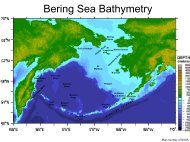
The objective of the Arctic Ice Dynamics Joint Experiment (ALDJEX) is to reach a better understanding
of the interaction of sea ice with the environment [l]. The main field experiment
ended in Play 1976 after one year of data collection on the Arctic Ocean. Data buoys were used
to define the motion of ice on the perimeter of the area of interest and to measure the surface
barometric pressure over the same area (Fig. 1).
2. Data Buoys
2.1. Data Results
A pilot experiment was conducted on the Arctic Ocean in the springof1972, during which data
buoys made detailed measurements of barometric pressure to develop and test atmospheric boundary
layer theories in preparation for the main experiment. An array of buoys which operated
for a year after this experiment provided drift and surface pressure and temperature data whic3
were also used to plan the main experiment [2].
During the 1975-1976 experiment, time series of position and pressure were obtained from a rix:
of 6-8 sites with accuracies adequate for numerical modeling. Two months of these positiondars
were accurate to 100'meters.
An array of buoys with about 100-kilometer spacing along the coast of the Beaufort Sea providcl
position data needed to interpret shore effects on the main array. These buoys should last
through 1976 and, together with the buoys further from shore which should last until 1978, will
provide data valuable to ice research and forecasting along the north coast of Alaska.
2.2. Development Results
Six types of sea ice buoys have been developed over a period of five years. Each has unique
features which have met data collection requirements and contributed to the evolution of new
designs. The principal characteristics of each are given in Table 1. Actual field experience
with these buoys and the technologiecincorporated in them now totals about 30 buoy-years and
is increasing at a rate which makes full evaluation of hardware performance and data very difficult
(Fig. 2).
-Six Arctic Data Buoys were deployed in 1972; four of these lasted about one year. The longesr
life was 667 days and the longest drift track was 1800 kilometers. This was the first use of
a lowpower satellite link, the Interrogation, Recording and Location System (IRLS),forposit;icn
and data retrieval. The spar configuration of this buoy was successful and has been used extensively
since. Experience with this design led directly to later RAMS buoy use [3].
Four of five Short Range Arctic Measuring Stations (SHRANS) operated 40 days in 1972 and provided
a detailed record of barometric pressure which led to revised sampling on later buoys arJ
to better field calibration procedures for barometers [4].
Eight HF-WavSat buoys were deployed in 1975 and lasted for 60 days. Four of these lasted 11
months. They raised the capabilities of sea ice buoys to a new level, with complete independ- ,
ence from experimental satellite systems. They featured the only operational use of fullaccuracy
Navy Navigation Satellite System fixes for data buoys. The high-frequency radio link
was married to both the 3- and 12-day memories in the buoy to successfully overcomearctic radir,
propagation conditions. A fully automated command, control and data reduction facility prove:
its value in data collection over a full year. Data gaps in the winter emphasized the need fir
an alternate communications frequency, which was disabled when the antenna could not be properLy
tuned in the available time. Corrosive failures in the electronics point totheneed for better
sealing from the humid summer sea ice environment. Two different pressure sensors were used
and should make it easier to isolate errors [5].
Eight of ten Synoptic RAMS (SYNRAMS) buoys deployed in 1975 before the Nimbus VI launch workei
and were among the first buoys acquired when the Random Access Measurement System (RAMS) was
activated. These buoys featured the first synoptic sampling and memory to work througha
7

poizr-orbiting satellite, which is important where uniform samples are needed and satellite
co~~erage is poor. This pointed the way toward fuller exploitation of the RAMS dnta capacity
I6l-
TWO of four Meteorological and Oceanographic (Met-Ocean) buoys operated for four months and one
coiitinues to work after seven months. A 3Gsecond transmission interval coupled with platfor;?
address switching extends the RAMS data capability to 64 bits per minute. Current speed and
directlon at two levels in the mixed layer and magnetic buoy azimuth are measured.
FiEteen Air-Droppable RAMS (ADRAMS) buoys have been deployed and all continue to operate after
a maximum of six months. The small electronic and battery package designed to withstand the
extreme Arctic surface environment, coupled with parachute deployment, has revolutionized ice
buoy deployment logistics.
3. Barometric Pressure Sensors.
Recent progress in other areas has been so rapid that the major technical challenge to remote
dnta collection is the need for better sensors. Our experience with barometers does not contradict
that conclusion, Our use of pressure sensors is perhaps unique in that we are able to
revisit buoys to perform calibration checks relatively easily 143. The preliminary resultsfor
a small sample of the pressure sensors used in the past year show that the Hamilton Standard
vibrating steel cylinder transducers drifted 0.1 millibar or.less during the year. There appears
to have been drifts in the reported buoy pressures measured with the Paroscientific vibrating
quartz beam transducers of from 1 to 4 millibars, but recalibration of the sensors in the laboratory
shows drifts of from nil to 0.7 millibars. The cause of this discrepancy is not unders:ocd
at this writing, but the possibility of an anomaly in the buoy electronics exists and
Yhould be a reminder that good transducers do not guarantee good measurements.
T!ie outputs of the barometers in use vary about 10% over full scale or about 1% over 100 millibars,
Thus, 0.1 millibar is one part in lo5 of the transducer output. Clocks in buoys must
56 better than one part in lo5 to avoid errors from this source. Also, synoptic sample timing
requires an accuracy of one part in lo5 to be good to 5 minutes per year. Cursors in the data
QT mode bits can permit calibration of the sample clock referenced to the satellite clock for
synoptic systeas. Where real-time sampling is used, the buoy clock can still be calibrated if
the buoy transmissions are controlled by the main buoy clock, including the unmodulated carrier
por:ion of the transmission. This method of controlling transmissions may also have benefits
in enhanced positioning schemes, and has been implemented on ADRAMS.
4. MRS Position Fix Accuracy
In order to provide a basis for the interpretation of the position fixes of the 25-30 drifting
RAMS buoys now in use in the Arctic Ocean, a study of aMS position errors has been made.
XL3)3EX receives data from NASA in the form of copies of the Nimbus archive magnetic tape with
S.~ion resolution of the order centimeters and various supplementary information including
satel;.ite position data and reference platform fixes.
&,is 4long-Track Errors
ExaEination of the fixes of RAMS platform 1337, located on St. Lawrence Island in Alaska, shows
"1e radial error (68th percentile of the radial distribution) varies from 2 to 6 kilometers
(Fig, 3). The RhVS system specification of 5 kilometers is met or exceeded for about 85% of
;he weeks analyzed over a six-month period. The error pattern of a reference platform operatel
by KASA near Fairbanks is nearly identical to that of 1337, which suggests that the errors are
from the same source; in this case, errors in the predicted satellite orbit. In fact, NASA has
identified irregul-arities in the along-track motion of the satellite to be the major source of
Ehese correlated position errors, and the along-track error component of reference platform
fixes is monitored on a daily basis to permit corrections to the orbit predictions. Since the
present method of operation relies on operator analysis of error trends, detected errors only
serve to improve the assumed orbit for future fix computations. The typical error growth and
correction pro.cess occurs over periods of a few days, so that the weekly statistics reported
here tend to average the worst events.
It is possible to use information on position errors of reference platforms directly to correct
oositions of moving platforms. This can be done either by adjusting the fix of a moving platfcrc!
with the error in latitude and longitude for the same pass of a reference platform, or by
reso!.ving the error into along-track and cross-track components prior to the adjustment. The
latter method requires information on the satellite orbit which is not normally provided to
xsers, but it does have the advantage that it is not affected by changes in the relationship
8

etween the satellite sub-track and the latitude-longitude grid between the two platforms.
Over a separation of 1000 kilometers both methods give essentially the same improvement and
result in radial errors below 2 kilometers most of the time (Fig. 3).
NASA could make an improvement in the positioning accuracy of RAMS, and save the user community
a lot of extra work, if the along-track errors of fixed platforms were usedto correct the fixes
of moving plat€orms. Similar arrangements should be made to improve Tiros N data, preferably
by using reference platform information to enhance the orbit estimates, rather than by the
direct adjustment of fixes. This was suggested for RAMS in a NASA-funded study in 1972 [8].
__
It is interesting that the radial position errors left after removal of along-track orbit errors
show the NASA platform to be consistently better than 1337, which uses low costbouy electrazics
and is exposed to large temperature fluctuations. There are significant periods of time whcr?
the NASA platform radial error is at or below 1 kilometer, which is in good agreement with
theoretical studies and which probably represents the best that can be done without enhancii;g
the actual time and frequency measurements made in the spacecraft [9]. With high quality pktform
hardware and implementation of software modifications the positioning accuracy of RAMS
could probably be brought to about 500 meters.
4.2. RAMS Fix Editing
The accuracy figures quoted above include all fixes reported by NASA withoutanyediting. Wkile
correction for along-track errors is more effective than any edit scheme we have tested as protection
against systematic errors, there are editing schemes which do seem to be selective L-
eliminating bad data (Fig. 4). All editing schemes make a compromise between eliminating bat
data and preserving as many fixes as possible. The quality index provided by NASA and the
ber of messages used in the fix computation perform better than the other edits in this regzrd.
After either of these edits about 80% of the fixes remain and the radial'error of the editel
data is about 50% of the unedited errors when along-track errors are not eliminated, and abxt
75% when along-track errors have been removed. Edits which might also prove effective when
data from two passes are used in the fix, but which we have not tested, are those which detect
unrealistic velocities or large differences between the two bias frequencies.
About one-third of the fixes have larger errors than the numbers given here as the 68th percentile
radial error statistic. If one has enough information about the limits of motiori of
the platform, then other editing schemes can be derived which eliminate the unreasonable date.
In our case, since we get about 10 fixes per day for each platfom., and the ice usually moves
less than 10 kilometers per day, the only editing used other than along-track error correcticn
is a running median filter. A more sophisticated Kalman filter is then used to produce the
final position and velocity estimates based on the RAMS fixes [lo].
5. Assessment of Polar Satellite Data Collection and Tracking
The primary advantage of data collection and tracking through a polar satellite system such As
RAMS is platform simplicity. This feature makes possible high platform reliability with low
cost. Those who are familiar with other more complicated satellite data collection and tracking
systems can hardly mistake the message of widespread use of W S .
The HF-NavSat buoy array cost about $800,000 more than the same spatial array of RAMS buoys 236
was less reliable. If the HF-NavSat buoys had been as reliable as the EtAMS buoys, the cost cf
a one-year experiment would have been about $250 per buoy-day versus $50 per buoy-day for t'kt
RAMS buoys. The €IF-NavSat buoy positioning accuracy of 100 meters was valuable to AIDJEX; 3-i
the compelling reason for these buoys was that we had to have data even if Nimbus VI didn't
survive. Rams buoy simplicity is made possible by total rel&"e,on a satellite system whick
is neither simple nor cheap. Users should familiarize themselves with the total system; not
just the buoys and the data package received from NASA. The active participationof aninforLc3
user community in full partnership with space organizations is essential to real progress.
As buoy costs approach $10 per buoy-day, the cost of sensors (and their simplicity and reliability)
becomes an important consideration. Taken one step further, the cost of data processiq
becomes a major factor. These are signs of progress since no one is really after buoys or
sensors, but data. Careful planning should include the cost of finished data. Data is the
realcurrency and the exchange rate is improving.
6. Satellite System Flexibility Concepts
The random access approach offers flexibility in data collection capacity and positioning accuracy
at the user's option. A normal real-time sampling system transmits about 300 bits of data

t@ the spacecraft during each orbit. The spacecraft memory can be used as an extended buoy
memory to permit the integration of multiple one-minute samples into ten-minute averages. i .-.e
treatmcrit of each data reception at the spacecraft as independent allows the use of multiplc
addresses and higher than nominal transmit duty cycles to obtain increased da ta capacity ..?Ti ::-.
no increase in equipment costs. The availability of up to 13 sntelljte passes per dav in i)b-:z~
regions means that up to 4000 bits per day can be transmitted for each address. There is
trade-off between the nrimber of data bits and level of redundancy required, and the nu::ber PI
satellite passes available and number of addresses used for each platform. This trade-cif I :-
a function of latitude, and with the number of passes available in polar regions we hi17.e h
extremely conservative with respect to data redundancy in our system designs. This should ch2:;e
as we become more confident of system performance.
Flexibility in position accuracy requires that measurements made in the satellite have sufficient
accuracy potential for the most demanding users. To achieve refraction-limited posit
accuracy of 200 meters, a Doppler system like RAYS needs measurement accuracy of 0.1 Hz and
0.61 seconds, an order of magnitude better than RA". The use of multiple addresses offers
the possibility of increasing the amount of data used in the position computation, as a way :f
improving fix accuracy. The flexibility offered to the user by random access data collecticx
and positioning systems should be retained and enhanced in the future.
7. Real-Time Data Readout Option
The Ni.mbus spacecraft transmits all data in real time in addition to storing these data on rzznetic
tape. When the spacecraft is critiiin view the data can be receivedwit'nportable equip.-::t
and, with the proper formats, can be decoded and interpreted essentially the instant they arc
transmitted from the platform. The most obvious use of this capability for data buoy work is
to provide for inmediate verification of platform performance during checkout of electrcnics.
This is the only practical method of authoritative confirmation of buoy pcrfor;nance in remozt
areas.
The same capability could be used to obtain data for forecasting without waiting for process5r;g
by NASA.
The primary purpose of this real-time data transmission is to provide a backup data collect
mode in case of tape recorder failure in the spacecraft. The spacecraft must be in view of
both the platforms and the data retrieval site for sufficient time to recover the desired dzr3,
Thus, the data retrieval site should be in the vicinity of the platforms, which is of specic:
significance to experiments in remote areas where NASA does not maintain facilities. The us?
of buoys in the Southern Ocean might be one experiment which would benefit from a direct re;;-
QUt capability in the Antarctic in the event of a tape recorder failure.
An important addition to the real-time data transmission of the spacecraft would be the predicted
orbit parameters and measured satellite clock and orbit errors needed for position fi-:
computation. This would permit fix computation by users and wou1.d make possible dispersing
the data processing function around the globe to areas where the data are being collected ar-i
used.
8. Conclusion
The data buoy program associated with AIDJEX has been large and diverse enoughtogainanapprsciation
for the many practical difficulties involved in developing and using several kinds CT
data buoys. Time seems to have been the ingredient in shortest supply, and should t?,ereforn
be canserved in future work. The money spent (about $2 million dollars including logistics
costs), while not extravagant, must certainly be considered adequate for the objectives, whi:i
were fairly well sati.sfied. Personal initiative was important, and more of this ingredient
would have improved the results.
We have been fortunate to try many new things with very few failures, but this should not bs
interpreted as an endorsement of the policy of trying something new when a proven method car.
be made to work. The only good pressure sensor is a used one. This is a good philosophy frz
buoys as well, althoush one probably has to settle for used designs and long checkout tests
since hardware recovery is difficult.
The RAMS has 2 to 6 kilometer position accuracy and is probably capable of 500 meters. By
taking full advantage of the flexibility available through random access, a data capacity of
one to several thousand bits per platform per day can be acheived. There are real benefits 10
be achieved through real-time readout of data from the spacecraft. These proven captbilities
of FUtIS, plus the potential ready to be realized, make it highly desirable that a new
I
10

deployment of the RAMS be scheduled so that the system can be utilized through the rest of :his
decade. A new orbit complementary in time to the existing one would be desirable.
Data collection and tracking from orbiting spacecraft is in its infancy. By comparison the
Navy Navigation Satellite System (Transit) has been an operational system for 14 years, and
currently consists of six Satellites which provide users with a completely self-contained pcsitioning
capability. The insight gained in the use of this system has lead to a new satellite
system which will provide continuous position information to a few meters, from a constellarion
of up to 24 satellites. The message is not that we need 24 data collection satellites. Ths
current concept of data collection and tracking is elegant in its simplicity. The challeng-. is
to raise our level of sophisitication in using the data collection and tracking concept tohigher
levels where even greater benefits will be realized.
9. Acknowledgments
This work was supported by the National Science Foundation, the Office of Naval Research, the
National Oceanic and Atmospheric Administration, the Bureau of Land Management, the Canadiaii
Polar Continental Shelf Project, and the National Aeronautics and Space Administration. We
wish to thank the staffs of the Nimbus Operations Center, Goddard Space Flight Center; Polar
Research Laboratory, Santa Barbara; the Applied Physics Laboratory, University of Washingtoz,
and our colleagues at AIDJEX.
10. References
[l] N. UNTERSTEINER, AIDJEX Bulletin 26
[2] P. MARTIN, in: Means of Acquisition and Communication of Ocean Data, WMO No. 350, 1973.
[3] D. P. HAUGEN and K. M. DOZIER, Applied Physics Laboratory, University of Washington,
APL-UW 7422 (1975).
[4] W. P. BROWN, AIDJEX Bulletin 22 (1973).
(1974).
[5] W. P. BROWN and E. G. KERUT, Ocean 75, IEEE Publication 75 CHO 995-1OEC (1975).
[6] S. P. BURKE and B. M. BUCK, Ocean 75, IEEE Publication 75 CHO 995-1 OEC (1975).
[7] P. MARTIN, Ocean 74, IEEE Publication 74 CHO 873-0 OCC (1974).
[8] Nimbus F TWERLE Doppler Data Processing, General Electric, Space Division No. 72SD4257
(1972).
[9] T. GREEN, Geoscience Electronics, GE-13, No. 1 (1975).
[lo] A. S. THORNDIKE, AIDJEX Bulletin 24 (1974).
11

BUOY NAHE
COMMUN. COMMANDS FIXES
TABLE 1. DATA BUOY CHARACTERISTICS
' NOMINAL
BITSIDAY X BATTERY TYPE NO. BUILT/
SAMPLING REDUNDANCY SENSORS f CAPACITY STRUCTURE TOTAL COST
5
A
k
rt
ri
P,
Arctic
Data Buoy
IUS
Nimbus
Beacon 2-5 km Real time
turn on IRLS 6 orblday
Rangerange
343 x 3 Pressure
Temperature
Voltage
Mercury
Polyethylene
3 KWH Spar buoy
7
$150.000
SBRAMS
VHF
Aircraft
Transmit None
data
Hourly 240 x 2 Pressure
24 orblday
Lead Acid PVC tube
0.7 KWH external
antenna +
battery
7
$100 000
P
N
HF-N avSat
HF- 4HZ
Beacon 100 meters 3 Hourly 1632 x 8
transmit NavSat 8 orblday + Colaaand
+ sample Doppler + Command
clock
shift
Pressure
Temperature
Volt age
Position
Zinc-Carbon-Air
Polyethylene
+ Lead Acid + Aluminum
45 KWH 4-leg spar
buoy with
aluminum upper
s truc tute
10
$1 0oo.Ooo
SYNRAMS
RAMS
Nimbus
None
1.5-5 ken
RAMS
Doppler
3 Hourly
8 orblday
256 X 15
Pressure
Temperature
Ambient noise
Zinc-Carbon-Air Aluminum spar
1 KMH buoy
11
$140 000
Me t-Ocean
RAMS
Nimbus
None
1.5-5 ~UI
RAMS
Doppler
3 Hourly
8 orblday
512 x 15
Pressure
Temperature
Voltage
Azimuth
Current speed
+ Direction
Zinc-Carbon-Air Polyethylene
1 KWH spar buoy
4
$104 000
ADW
m
RAMS
Nimbus
None
1.5-5 km
RAHS
Doppler
Real t b e
10-12 orb
f day
352 x 11 2 buoys with
Pressure
Temperature
Inorganic
Lithium
1.5 Kwtl
Lexan
sphere
17
$192 000

(Martin & Gillespie)
Fig. 1. Initial and final array of buoys for AIDJEX main experiment,
June 1975-May 1976: 0-0, initial array; 0-0, final . _ _ "
array;, 0 , additional buoys.
20
.
15
Estimate
5
* I
I
I
i
'71 '72 ' 73 '74 ' 75 '76
Year
Fig. 2. Accumulation of data from buoys during AIDJEX, 1971-1976.
13

L(
0 I 2 3 4 3
Radial error, kilometers
-/.
?ig. 3. Effect of various editing techniques on ?AIS accuracy with
and without along-track errors for NASA reference platform, 15-
20 Feb. 1976. Lower case--along-track errors are present: upper
case--along-track errors are removed. Type of edit--8 = none;
A = elevation angle; B = messages used > 12- C = messapes used
> 8; T = two pass fixes only; F = A+T; Q = quality inclex .? 47.
H = A+T+q.
r l
i-? ~
Improvement in TMS ~osition errors by removtnp ?Xong-tracL
satellite errors. IB platform 1337, mcorrected: t platforr; 1237.
corrected; NASA platfom,, corrected,
14

Arctic Environmental Buoy System
Walter P. Brown
Polar Research Lab., Inc.
Edmund G. Kerut,
NOAA Data Buoy Office
ABSTRACT
The AEB is a remote unattended data acquisition
and telemetry system designed for deployment
on ice covered seas. The total system as
presently configured consists of up to 12 AEBs
and a Central Control Station (CCS). The Central
Control Station under computer control
collects the data from the AEBs, processes the
data and formats the data on a digital tape for
future analysis. The CCS is also capable of
controlling the majority of the AEB functions
via a command link. The AEB is configured to
sample sensor data and acquire position data
at three hour intervals automatically. The
present sensor configuration allows 6 primary
sensors with 10 bit resolution and 16 auxiliary
sensors with 5 bit resolution. The auxiliary
sensors are sampled only once per day. The
sensor data and position data are stored in a
digital memory which is transmitted via an H.F.
link once per day to the Central Control Station.
A unique dual memory concept is utilized
to prevent data loss due to propagation vagaries
and polar cap absorption events. The
position measurements are accomplished by an
on-board NAVSAT receiver.
INTRODUCTION
The NOM Data Buoy Office (NDBO) engineering
development activities include the development
of arctic data buoys in support of national and
international scientific experiments. As part
of these activities a program has recently been
successfully concluded to develop and test three
prototype arctic environmental buoys (AEB) to
provide the remote data requirements of a
scientific experiment designed by the kctic
- Ice gynamics Joint Eperiment (AIDJEX) Project
Office. The experiment is designed to investigate
the large scale response of sea ice to
changing environmental parameters. The AIDJEX
program as presently envisioned is the first of
a series of studies that will subsequently be
incorporated under a large E a r seriment
(POLEX). The objective of the AIDJEX experiment
is to reach, through coordinated field experiments
and theoretical analysis, a fundamental
understanding of the dynamic and thermodynamic
interaction between arctic sea ice and its environment
and to answer basic questions of the
mechanisms which cause large scale ice deformation
and the effect of ice deformation and
morphology on the heat balance.
The experimental design requires the establishment
of an array of drifting ice buoys in the
Arctic Ocean to measure atmospheric pressure and
temperature at the sea ice surface. An essential
requirement of the buoy design was to develop a
position determination capability, an order of
magnitude beyond the capability of polar orbiting
meteorology satellites with position fixing capability,
which would be operational during the
experiment .
The program phases included the following
elements: the study of the experimental design
for the AIDJEX experiment which involved the
array of Arctic Data Buoys (AEB) and the translation
of the system measurement requirements
into a system specification; the design and
development of prototype system hardware to meet
the measurement requirements and test objectives
of the AXDJEX experiment; fabrication of three
prototype AEB's and associated test set for test
and evaluation in the field prior to the main
experiment; and performance of laboratory and
field testing on the prototype system to verify
experimentally its ability to meet the measurement
requirements and test objectives of the
main experiment. The design, development and
fabrication program was performed by the Polar
Research Laboratory in Santa Barbara, California
under contract to NDBO.
DESIGN CONSIDERATIONS
The conceptual design of the Arctic Environmental
Buoy (AEB) System was formulated to meet
both the near term requirements of the Arctic Ice
Dynamics Joint Experiment (AIDJEX) and the general
need for gathering data on the Arctic ice
pack. The basic requirements were to sample a
number of sensors on a synoptic basis (i.e.,
every 3 hours starting at 0000 Zulu), provide an
accurate position for the system 8 times a day
and to transmit the data at least once per day.
In addition the AEB system was to have an unattcnded
life of 8-14 months. The range of the remote
buoy stations from the Central Station is expected
to be 250 to 500 Km during the life of the
experiment and therefore an H.F. link was selected.
Frequency selection and modulation methods
were chosen on the basis of computer analysis
and studies (1)(2)(3) performed at the Institute
of Telecommunication Sciences in Boulder, Colorado.
The structural design of the buoy hull and
antenna was heavily influenced by the unique
environmental conditions of the Arctic ice pack.
50 - IEEE OCEAN '75
15

The buoy will be subjected to temperaebres as low
as -5OOC in the winter with ictemit- ng
and temperatures of + 5OC in tbe rumer w
moist air and the possibility af flee floating,
In addition the structure must be able LG dthstand
the loving attentions of a polarr iear,
The Navy Navigation Satellite (NAVSA
selected for positioning becat'se o_C
ly good accuracy (sjometers radius CEP, sirqie
channel, co-location mode) and tPac eacc posf.tio~~
fix defines a unique position ma !s ?cr depe?-
dent on past history (lane counting) a8 is
required in OMEGA or Global positim systems.
The emphasis in the design was piaced os conserving
power and weight and in ~rovidhg redmdancy
in high risk areas. The volume ai.d weight
of the system had to be compatible ?dth tFe
capabilities of a Twin Otter aircrait.
AEB SYSTEM DESCRIPTIOE
The AEB system consists of 8 remote statiovs
installed in a circular pattern with a radics ot
300 to 400 kilometers from the central ALDJEX ice
camp. These AEB's are received and interrogated
by a Central Control Station (CC3) locaze? st the
central AIDJEX ice camp. The AEB is a self contained
unmanned telemetry statior. installed in
the ice pack with a battery ?over suppLy capable
of 14 months of continuous operatior., As presently
configured the AEB's sample 60 bits (if
envirorxnental data and 144 bits of pcsitior
information every three hours. Addit'iora!.
environmental and position samples caq 30 c0-f
manded from the Central Control Station. R e
AEB environmental sensor suite for AXDJEY consists
of two atmospheric pressure senccrs and
two temperature sensors, eacb. u~ing a 10 bi:
word, thus leaving 2 spare 10 bit sensor inputs
available.
The position samples are obtained frob6 Nav'-
gation Satellite receiver uhicl- provides GIE 24
bit word of identification data and fd7;e 24 blt
words of doppler data. Each of the sens3r and
position word groups has 48 bits of sync an?
reference information attached which ~c,~des a
5 bit sample of engineering data. The evvlrrxmental
data, engineering data and positLop data
are stored in two digital IC m~mories. 9-e maory
provides short term storage .sf 2 de 7c, "ata
and a long term memory provides 12 days. of stcrage.
The long term memory is used to c~vsr
communication link interruptions of t~r TO 12 Says
and to fill in holes fn daily transmissions. Two
cycles of the short term memory axe era?snit:ed
once per day and two cycles ot the lcng term
memory once per 10 days on an automatic basis.
Additional transmissions from eitber n%orv can
be commanded by the Central Contrct S"bat"o- The
AEB also contains a strobe light acZ 'XF beacon
transmitter as location aids. Tbes? ~n;e_s Ere
turned on automatically once per 13 days FoS
three hours and can also be turned ca by coaaand
from the CCS.
The Central Control Station prev%des for data
reception and remote control of the AZB's. Tt
contains a Navigation Satellite -eceivnr ;rnic\
is used to obtain local fixes and pr-v'des :\e
additional message data necessary to calc~late
M1B -osi:iccs. Received data is processed by e
Rous 2,i'lC computer whjcb mssages the raw AEB
sensor data into a finishel form and stores this
iafcrmation on a digital magnetic tape. Th2 conpriter
also provides control of the CCS operation
arid sends commands tc the AES's as required.
Srck-up Yecsrding of data is provided, in cese of
compxter faiiure. Ar. ,.ninterrL?tzhie power su?p€y
furnishes primary power to criticzl components so
chat data 5s not I=st d:;e :o t+,e frequent c,itPBes
:~f ice CZR~ power.
An Mi3 test set conc-aLns the ne-.essary eouipment
to test and isolate problems in the A9B to
aub-system level. Th.e.test set is also capable
of sendir.8 comands te and receiving data from
the AEB, thus simulating the CCS station.
AEB ELPCTRONIC DESIGN
W block liagrao of the AEB is shown in Figure
1, A11 sensors except the engineering sensors
are sampled qncc every 3 hours beginning at 0000
hours Zulu. Starting at the top, the NAVSAT receiver
is turned on €or one hour by the control
electronics. The receiver begins sweeping and
evectually locks onto a satellite. It then
"Lacks the satellite until message synchronization
is established. At this point it reqxests
the control electronics to send it the Zulu time
of day which it stores in an internal register.
Alsa it extracts the relative Zulx time and the
satellite I.D. Erom the -eceived message and
stor~s this infomation. It then continues
':racking che saifllite imtil five 2 minute
d.oppler intervals are received. At this point.
the NAVSAT receiver signals the memory and conrroP
sub-systeas that data is rcady. At :he
prcpes point ir. the memory cycle the data is
transferred from the NAVSAT register into the
memory. The ahcve description describes a normal
NAVSAT cycle. Additional logic within the NAVSAT
receivers allows for 2 other conditions. In one
case the receiver could lose RF lock on the
satellite before it had acquired 4 doppler neasuremenfs.
Uilde~ this condition if the one hour
gate .~K-!E the cortrol electronics is sti.11 high
the NAVSAT .receiver will begin swceying again
an? attempt to acquire another satellite. Ir.
s~.oti:er case if four dopplers ar
2.F lcck :s iost t:-e o7zrztlon wi
as in :he :icxzaP case and cn1.y 4
be stored whicn is sufficient for a position fix.
The time thc NAVSAT receiver is ON will vary
from 18.5 minutes to 1 hour. In general. hecausz
nf the high number 06 satellite passes in
thz Arctic the ON tiimr. should be less than 70
minutes on the average.
-.
;ne yressure se2sors are turned
a?.riutes at each s;moptic time. The
zf rb? eteven IS used to allow -he sensors to
stabilize, durlng the next PO minutes the outputs
OS %he pressu~e transducers are averaged. The
technique used is eo continuously count the
freqxency output cf the pressure trsnsducers in
a 10 bit counter and store the count at the end
of the 19 minute period. Because the barometric
pressure range of intcrest (SSO-lOSG nillibars)
Ls only Z~GV,: a 1/10 ?f the tranducer pressure
range, a suitable 6igital divider must be used

etween the output of the transducer and the 10
bit counter to avoid an overload problem. With
the 10 bit counter the barometric pressure resolution
is a nominal .1 millibar.
The two temperature sensors, the spare sensors,
and the engineering data sensors are all conditioned
to provide an analog output of 0 to -5
volts. The temperature sensors cover a range of
-50°C to +lO°C with a resolution of .06OC. These
outputs are multiplexed into a 10 bit AID converter
and except for the engineering data sensors
are dumped into the memory at each three
hour sample period. The engineering data sensors
are sampled only once per day with two of the
sensors being entered into the memory each three
hour sample period. Only the 5 most significant
bits of the AID are used for the engineering data.
The engineering data presently being measured are:
RF power out and reflected power; primary and
secondary battery voltages; several temperatures
in the electronics housing and a leak detector.
The short and long term memory are operated
identically except that the long term memory is
exactly 4 times longer than the short term which
contains 7200 bits of storage. Both memories
use dynamic MOS shift register chips connected
in a serial recirculating memory configuration.
Two types of words are entered into the memory;
a sensor word which is 108 bits and a NAVSAT
word which is 192 bits. The words are entered
sequentially and once the memory is filled the
new data replaces the oldest. The word formats
are shown in Table 1. Both the sensor and
NAVSAT words start with a sync pattern. This
approach uses more memory space for non-data
and requires more transmit time than a less
frequent sync pattern approach such as once per
day. However, it has the advantage of allowing
sensor and NAVSAT words to be entered randomly
with no word limit per day. It also has the
advantage on the receiving end of improving the
amount of data received. Fading is quite prominent
on H.F. links and if a fade occurs during
a sync pattern with this scheme only one'data
word is lost where with a less frequeny sync
pattern approach a larger block would be lost.
The short term memory is normally connected to
the Bi-phase L modulator and is transmitted on
a daily basis. Once per 10 days the long term
memory is switched into the modulator and transmitted.
Two VCTCXO's are supplied to provide
redundancy or the flexibility of dual frequency
operation if needed. The present plans call for
operation on a single frequency, therefore both
VCTCXO's are the same. In the event of a failure
of the VCTCXO being used, a command can be sent
from the CCS station to switch to the alternate
one. The VCTCXO's are passively combined and
either can drive the 100 watt power amp. The
power amp is configured such that either half
can fail and still allow degraded communication
with 25 watts output. The power amp is broadband
and will provide its full output over a frequency
range of 2 to 12 MHZ. A coax switch is used to
switch the antenna from the command receiver to
the transmitter during the transmit cycle. A
matching network is used at the base of the
sleeve dipole antenna to allow adjustment for
various ice thickness. The command receiver
operates on two frequencies to allow 24 hour
command coverage. The present assignments are
4.165300 and 2.146 MHZ. The control circuits
switch the receiver between these two frequencies
on a one minute cycle. This procedure eliminates
the need for two separate receivers and is acceptable
since none of the commands require immediate
action. To assure reception of the command
on the right frequency, the CCS station merely
sends the command sequence twice with a one minute
spacing, The command is decoded and sets up
the required action in the control electronics.
Two location aid devices are provided. A 300
milliwatt VHF beacon on 108.1 MHZ allows an aircraft
to "home" on the buoy from a range of 30
to 50 miles. A strobe light allows visual sighting
of the buoy in twilight or dark conditions
with ranges up to 10 miles.
The AEB power supply consists of three banks
of primary carbon-air cells with each bank consisting
of fifteen 1000 amp hour cells. Because
of the nature of these primary batteries, they
are not capable of providing the peak current
demands of the system, therefore they are used
to charge a secondary battery bank. The secondary
battery consists of 36 Gates sealed lead
acid cells arranged in three 12 volt banks which
provide approximately 24 amp hours when fully
charged at O°C. Individual chargers are used
between the secondary battery banks and the
primary banks and the secondary banks are diode
isolated from the power buss. Thus, a failure
in any of the banks will not stiut the system
down but will reduce the life of the system.
The master timing for the AEB is derived from
a very stable oven controlled 5 MHZ oscillator.
Typical stabilities for the oscillator are 1 X
10-9 per 30 days. In 14 months there are 10,224
hours, thus the error in time at the end of the
experiment using this oscillator should be less
than 1.0 seconds assuming that the above stability
is a linear change over the 14 month life
and that the frequency was properly set initially.
AEB STRUCTURAL DESIGN
The structure of the AEB as installed in the
Arctic ice pack is shown in Figure 2. In developing
the design full advantage was taken of some
of the unique characteristics of the ice cover
sea. The ocean water below the ice remains thermally
stable with only 2OC variation and a mid
point near O°C over the entire year (4). The
ice itself acts as an insulator against the surface
temperature extremes. Equipment installed
under the surface of the ice will never see
tehperatures lower than -2OOC even though the
surface temperature may reach -5OOC (5), (6).
These facts are utilized in the design by locating
all the electronics and the batteries below
the surface of the ice in 8" diameter tubes.
The electronics modules are located in the central
tube. The temperature sensitive components
such as the master oscillator and barometers are
located in the bottom of the tube which is surrounded
by the sea water. The other electronics
modules are placed above these in order of decreasing
temperature sensitivity. The electro-
52 - IEEE OCEAN '75 17

nics occupy about 12 feet of the 17.5 foot long
tube which extends 3 feet above the ice, Thus
the electronics are all below the surface. The
tubes extend 3 feet above the ice to prevent
possible flooding from melt ponds which xcur on
the ice surface in the summer. The primary batteries
are located in the outer 3 tubes and
occupy approximately 14 feet of vertical space
thus the batteries are also below the surface of
the ice. These tubes are the support for the
upper structure and provide enough buoyancy to
maintain the system at approximately the same
level even in a full melt condition.
The upper structure consists of 6 twelve foot
radials with their supporting arms; a 6 inch diameter
12 foot long sleeve which provides the
mounting structure for the temperature sensors,
the VHF Beacon antenna, the NAVSAT antenna, the
strobe light and acts as the feed line for the
H.F. whip antenna. The H.F. whip is 24 feet long
and is center loaded for the 4.1653 MHZ transmit
frequency. The abbreviated radial system was
used in an attempt to minimize the effect on
antenna impedance of possible shifts in the ground
plane due to summer melt condition. The chains
at the ends of the radials are used to dampen
wind-induced vibration. The antenna structure
was grounded to sea water through the battery
tubes. The temperature sensors are located
nominally at 1 meter and 3 meters above the ice
surface in radiation shields attached to the
sleeve. The strobe light, NAVSAT antenna and
VHF Beacon antenna are spaced120' at the top of
the sleeve to minimize structural interference
effects and to improve line of sight range.
DEPLOYMENT
The AEB's were deployed using a Twin Otter
fixed wing aircraft equipped with skis. A multiyear
ice flow in the desired location was selected
and reconoitered for a suitable landing site.
After landing,small pilot holes were drilled to
determine ice thickness. If a suitable thickness
of 8 to 12 feet were found, the installation was
begun. Holes were drilled thru the ice for the
four 8" diameter tubes using a 9" ice drill.
The tubes were installed and the primary batteries
loaded into the outer tubes using a tripod.
These primary batteries could not be pre-loaded
prior to installation because they are wet cells
and could not be carried horizontally in the
aircraft. The central electronics tube was preloaded
however, and was placed in operation prior
to leaving the AIDJEX main camp. The electronics
were running on their internal secondary battery
bank, in some cases continuously for 3 weeks,
prior to deployment. This procedure obviated the
need for turn-ON and extensive checkout in the
field. While the tubes were being installed the
upper antenna structure was being assembled. The
upper structure was then placed on the tubes and
electrical connections were made between the
electronics tube and the batteries and antennas.
A brief check was then performed to be sure that
the H.F. transmitter, NAVSAT receiver and
Location Aids were operational. Installation
time averaged about 3.5 hours with a 3 man
installatlon team and occasional assistance from
the pilots. The installation of 8 AEBs was
accomplished over a period of two months with
the biggest delay due to weather. Their approximate
positions along with that of the AIDJEX
main camp are shown in Figure 3.
CONCLUDIHG REMARKS
Eight AEBs are now operational on the Arctic
Ice Pack. These buoys are presently being used
to gather data necessary to finalize a mathematical
model of the ice pack. As such, they provide
barometric pressure temperature and position data
on a 3 hour synoptic schedule at a fraction of
the cost of manned camps at similar locations to
gather data. The AEBs have been designed with
the flexibility to easily adapt to a wide variety
of other sensors and can be used wherever periodic
data over a long term is needed.
The design and development of the AEB system
and three prototype buoys was funded by the NOAA
Data Buoy Office and the fabrication of the
remaining AEBs and the Central Control Station
was funded by the National Science Foundation
through the AIDJEX Project Office.
ACKNOWLEDGEMENTS
An essential feature contributing to the
success of the program was the close liaison and
engineelring and scientific contributions by the
AIDJEX staff members during the development
phases of the program. In particular a debt of
gratitude is owed to Pat Martin, the AIDJEX
technical coordinator, for his dedication in
reviewing and critiquing the design and for his
devotion to the difficult task of completing the
installation of the 8 AEBs in the Arctic ice pack.
REFERENCES
ITS Propagation Studies for Polar Research
Lab DTD 10123173
AKIMA, H., "Modulation Studies for IGOSS",
ESSA Technical Report ERL 172-ITS 110,
June 1970
Hatfield, D. N. and DeHass T., "System
Design Considerations for the Development
of the IGOSS Ocean Data HF Transmission
System", ESSA Technical Report ERL 158-ITS
101, March 1970 .
Coachman, L., "Water Masses of the Arctic"
Proceedings of the Arctic Basin Symposium,
Arctic Institute of North America,,Page
145, October 1962
Maykut, G. and Untersteiner, N., "Numerical
Prediction of the Thermodynamic Response of
Arctic Sea Ice to Environmental Changes",
Page 54-57, Rand Corporation Memorandum
RM-6093-PR. November 1969
Brown, W. P., ''AIDJEX System Phase I,
Final Test Report for Ice Island T3 Antenna,
Battery and Structure Tests", Polar Research
Lab, Inc., Report TR005, October 1974
18 IEEE OCEAN '75 - !X3

Sensor Word
Description - Bits
TABLE I
Description
NAVSAT Word
sync 24 Sync
Buoy I.D. 4 Buoy I.D.
Julian Day # 10 Julian Day
Word I.D. 1 Word I.D.
Word # 4 Word #
Engr Data 5 Engr Data
Press Sensor #I 10 Buoy,Time of Day
Press Sensor 12 10 Satellite I.D.
3 Meter Temp 10 Re1 ZULU Time (SAT)
1 Meter Temp 10 Doppler Count 81
Spare $1 10 Doppler Count 12
Spare #2 - 10 Doppler Count 13
Total 108 Doppler Count 64
Doppler Count #5
Total
- Bits
24
4
10
1
4
5
14
5
5
24
24
24
24
54 - IEEE OCEAN '75 19

Ill --
- KEY
AIUJEX WIN WW
AEBa 0
4
4
VI
I
VI
VI
FIGURE 2
AEB STRUCTURE
FIGURE 3 AEB POSITIONS AT END OF SPRING 1975

AIR DROPPABLE RAMS (ADRAMS) BUOY
W. P. Brown
Polar Research Laboratory, Inc.
123 Santa Barbara Street
Santa Barbara, California 93101
E. C. Kerut
NOAA Data Buoy Office
Mississippi Test Facility
Bay St. Louis, Mississippi 39520
Abstract
The ADRAMS buoy was developed to provide
remote tracking of drifting sea ice near the
Arctic coast. The air droppable feature was
employed to reduce the high cost of deployment
inherent to manual installation and to provide
access to, deployment areas and seasons of the
year not previously suitable. ADRAMS contains
a 401.2 MHz transmitter and suitable digital
encoding to allow it to be received by the
NIMBUS-6 satellite. This satellite contains a
random access measurement system (RAMS) package.
The RAMS system determines the position
of the ADRAMS buoys to an accuracy of better
than 5 €31 thru doppler measurements of the
received signal. The buoy is deployed via its
own parachute and is designed to survive and
properly orient its antenna on any type of
terrain. The 80 pound package contains enough
batteries for 7 to 8 months operation at surface
temperatures as low as -5OOC. Although
the original ADRAMS was designed for tracking
only, it has been modified to incorporate a
capability for sensor data telemetry. The RAMS
system in the NIMBUS-6 satellite accepts 32 bits
of data from each transmission. Nineteen ADRAMS
buoys have been deployed thus far; 17 in the
Arctic and 2 in the Antarctic. The air drops
have been 100% successful.
1. Introduction
The Bureau of Land Management, in conjunction
with the Arctic Ice Dynamics Joint Experiment
(AIDJEX) program, developed an urgent need for a
device to allow remote tracking of the Arctic
ice pack drifting near shore. This need resulted
from the expansion of oil activities on the
northern coast of Alaska and from problems encountered
during 1975 in attempting to ship
large amounts of material to the oil-rich Prudhoe
Bay area.
Because of the urgent nature of the program,
it was probable that the buoys would have to be
deployed,during the all-dark period of winter
in the Arctic and under adverse weather conditions.
Previously-developed Arctic data buoys
(~,2) were not suitable because their installation
required a crew to land on the ice, an
operation too hazardous for the dark of winter.
21
Therefore, the concept was evolved for a small
buoy which could be deployed from an aircraft via
parachute. With the constraint of small size,
the obvious choke of a tracking scheme was the
NIMBUS-6 satellite Random Access Measurement
System (RAMS). This system is being used succese
fully in other buoy programs. The buoy was given
the acronym ADRAMS (Air Droppable RAMS). The
NOAA Data Buoy Office was selected to spearhead
this program because of its wide experience in
developing data buoys for the open ocean as well
as the Arctic.
A contractor, Polar Research Laboratory, of
Santa Barbara, California was selected to perform
the ADRAMS design, development, and fabrication.
2. Design Considerations
The following factors provided the major constraints
on the overall system design.
1.
2.
3.
4.
5.
6.
7.
8.
The fabrication of the first group of
buoys had to be complete within six months
of the program start to allow deployment
for the critical winter season. This
factor constrained the use of electronic
components, materials and energy sources
to those that were readily available.
The size of the buoy could not Cxceed the
dimensions of the parachute door on available
deployment aircraft.
The electronic subsystems and mechanical
structure had to withstand the landing
impact of a parachute landing on smooth
and rough ice.
The parachute had to be disconnected from
the buoy after landing to prevent the buoy
from being dragged across the ice by high
winds.
The rate of change of oscillator frequency
with temperature had to be minimized, wittr
out using power, to optimize tracking
accuracy.
The system was to have a minimum life of
six months.
The system was to withstand the
surface temperature extremes of
-5OOC.
ice pack
t10 to
The buoy hull had to be water t ght in the

event that a melt pond should form around
the buoy during the sumncr.
9. The antenna was to remain horizontal
regardless of the landing attitude.
10. The cost was to be minimized since the
buoys must be considered expendable.
Individually, none of the above factors was
difficult to achieve, but taken together they
presented an interesting design problem, The
requirement for completed buoys in six months
posed the biggest difficulty in that time did
not permit testing a variety of approaches prior
to freezing the design. Fortunately, the selected
approach proved satisfactory; the buoys were
delivered in time and deployment was 100% successful.
3. System Description
A sketch of the ADRAMS buoy is shown in Figure
1. The buoy consists of a 22-inch diameter polycarbonate
sphere mounted on a 15-inch diameter,
12-inch high foam crash pad. The electronics,
antenna, and battery pack form a single unit
inside the sphere and are free to rotate around
both vertical and hcrizontal. axes on teflon bearings.
The electronics module contains a pendulus
weight so that after deployment, regardless of
the final resting position of the sphere, the
antenna will be properly oriented for optimum
satellite reception.
The system is powered by newly-developed
inorganic lithium batteries. These batteries
have extremely high energy density on a weight
and volumetric basis and allow operation down to
the -5OOC temperature limit of the system. The
battery pack weighs less than 9 pounds and provides
an expected life of 7 to 8 months.
A special ruggedized BTT (Buoy Transmit Terminal)
was developed to survive the shock of an
air drop as well, as the low temperature extremes
of the Arctic ice pack. The electronics were
bui1.t in modular form to facilitate expansion and
-to allow adaption to other form factors. In
addition, a "modified canted turnstile" antenna
was developed from a design for the SYS satellite
(3). This antenna provides circular polarization
and has a low vertical profile consistent with
the buoy's spherical configuration. Pictures of
the various elemenzs of the buoy are shown in
Figure 2.
In operation the buoy transmits a signal for 1
second each 62 seconds with a nominal radiated
power of 31 dBM. The format of this transmitted
signal is shown in Figure 3. A zero phase reference
signal with no modulation is sent for a
nominal period of 350 msec. During this period,
the NIMBUS-6 satellite acquires phase lock and
establishes its phase reference. The next
approximately 640 msec of the signal contains the
message and is phase modulated t60° at a bit rate
of 100 Hz. The first 30 bits of the message contain
the bit sync and frame sync followed by the
platform identification number. The next two
bits are used to provide up to 4 variations on
the 12 bits of data which follows.
The NIMBUS-6 Satellite is in polar orbit, COT"-
pleting one revolution of the earth approxinatclv
once each 108 minutes. The number of orhits
which are in view of a platform on the earth's
surface varies with the platform latitude. i'uur
to six passes a day are typical near the equator
to 11 or 12 passes near the poles. The number
of "hits" (received transmissions) per pass also
varies, depending on the elevation angle from
the platform to the satellite at the closes point
of approach. The variation in hits is typically
3 at low elevation angles to 15 at high elevation
angles. To achieve :he stated accuracy (55 L'l)
of the NIMBUS-6 tracking system, at least two of
three consecutive passes must be received with at
least 3 hits per pass (4).
4. Electronic Design
A block diagram of the electronic subsystem is
shown in Figure 4, The oscillator is a temperature
compensated crystal osciliator (TCXO) at a
frequency of 3.134375 1'Mz. A higher frequency
crystal could have been used, with less postmultiplication
needed, but the 3 MHz crystal is
inherently more stable and easier to compensate
over the required wide temperature range. 'The
3 PMz oscillator signal is multiplied to 50 PIHz
in a X16 multiplier and then to the final 401.2
MHz carrier frequency with a X8 multiplier. The
carrier signal is then phase modulated by the 3-
state phase modulator. The phase modulator uses
a hybrid coupler for ease of impedence matching
and uses pin diode switched transmission lines.
Individual 10 volt logic levels from the COSPIOS
digital logic selects the phase state as Oo, 60'
or -6OO. The phase modulator drives the power
amp, which is a single chip hybrid circuit capable
of up to 2.4 watts output. The digital
encoder and timer generates the bit sync, frame
sync and platform I.D. as MkVCHEZTER CODED 100 Hz
data which is applied to the +60 phase modulation
inputs. It also generates a 0' phase signal
at the beginning of the transmit cycle for 350
msec. The timer portion of the digital module
contains a crystal oscillator and countdown
circuit to generate the basic transmit timing
cycle of one second per 62 seconds. The one
second transmit gate is applied to the power
switching and regulator circuit which provides 3
switched regulated voltage to the multiplier and
power amplifier stages.
The battery supply provides continuous power
to the TCXO and Digital Encoder and Timer. These
two units have an average drain of 12.7 milliamps.
The remaining units have an average drain of 7.3
milliamps with their 1/62 duty cycle. The total
average drain is 20 milliamps. Five parallel
banks of 4 inorganic lithium cells in series are
used as the battery supply. These cells are a
relatively new development by General Telephone h
Electronics Laboratories. They are hermetically
sealed and therefore do not have the SO2 corrosion
problem of the more common organic lithium
cells. They provide very high energy on a weight
and volume basis with reliable operation well
below the required -5OOC. The cells weigh 6.5 oz,
have a terminal voltage of 3.6 volts, a flat discharge
characteristic, and a capacity sf 22 amp
22

hours. The twenty-cell battery pack has a voltage
of 14.4 volts and a capacity of 110 amp hours.
A single additional cell is used to provide
switch and regulator bias. Expected life from
the above pack is 7.5 months.
The antenna is a modified canted turnstile
antenna which provides right hand circular polarization
and good hemispherical coverage. It consists
of four quarter wave vertical stubs canted
45O tangentially around a half wave diameter
circle. Each of the stubs is fed 90' out of
phase with the preceding one, progressing around
the circle.
Although the original ADRAMS was designed for
tracking only, there was soon a requirement to
add a data capability. Several units were modified
to incorporate a precision barometer and an
internal temperature sensor. Both sensor outputs
were converted to 10-bit digital words and interfaced
to the digital encoder. The temperature
sensor range is +30° to -5OOC with better than
. l0C resolution. The barometer pressure range
is 950 to 1050 millibars with .1 millibar resolution.
Since the buoy had to be water tight,
a special teflon membrane was used for the
pressure port which allowed barometric pressure
changes to enter the buoy but kept moisture out.
5. Mechanical Design
The major mechanical tasks associated with
the development of ADRAMS included the following:
development of a subsystem for paradropping
ADRAMS and releasing the parachute after ice
impact; packaging the system to survive ice
impact; making provision for maintaining the
antenna in a vertical position regardless of
orientation of the overall package; and selecting
materials compatible with the impact loads
and sub-zero temperatures.
The mechanical design consists of four subsystems:
1) the inner gimbal which contains the
antenna and electronics; 2) the sphere which
houses the gimbal; 3) the impact pad which
-ahsorbs the shock of the landing and 4) the
parachute and its releasing mechanism. These
are shown in Figures 1 and 2.
Gimbal Subsystem
In order to maintain the antenna in a vertical
position, the entire electronics assembly was
designed as a pendulous self-leveling gimbal
revolving inside a 22" diameter sphere. Tlie
gimbal apprcach was found to be much simpler and
more reliable than attempting to deploy automatically
a fixed antenna in an upright position
on the rough surface of the ice pack. The gimbal
insures that the antenna will be vertical not
only upon,landing but also during any future
disturbances due to wind, ice surface changes
due to movement, melting or polar bear interference.
The weight of the entire gimbal including the
electronics, batteries and antenna is 50 pounds
and rests on 4 teflon bearings which are free to
slide over the inside surface of the sphere.
These bearings are spring-mounted onto the gimbal
allowing them to retract on impact. The deceleration
forces are then picked up by a polyurethane
pad which distributes the impact load
evenly over the bottom of the sphere.
The teflon bearings have a low coefficient of
friction but to further enhance the self-leveling
capability a lubricant was used on the inside
of the polycarbonate sphere. Several oils and
greases were tested for both lubrication and
freezing properties. A silicone base grease
was selected which has excellent lubricant qualities
to temperatures below -5OOC.
Buoy Hull
A number of materials and fabrication
approaches were considered for the outer sphere.
The antenna could not tolerate metals within
its pattern, so the sphere had to be non-metallic.
It also had to be capable of withstanding
the impact loads. Vacuum formed acrylic and
ABS plastic hemispheres were tried, but the
manufacturing technique produced a very thinwalled
apex (about 118") thereby reducing the
strength of the sphere. Polycarbonate plastics
were then investigated. These plastics have
about 16 times the impact strength of ABS and
40 times the impact strength of acrylics. In
addition they can be "rate-formed" to provide
a uniform wall thickness. Rate-forming involves
heating powdered resin inside a complete spherical
mold which is heated and rotated about all
axes. The result is a sphere with a smooth
inside s-urface. The sphere is cut in half and
fiberglass flanges are installed.
A teflon gasket material is used to seal the
two hemispheres. Caulking was rejected because
of the possibility of leaks into the sphere
interferring with the gimbal, Twelve 318" x 2"
nylon bolts are used as fasteners for joining
the hemispheres.
The flange Ltself is square-shaped instead of
round to reduce any tendency to roll in a wind.
Shock Absorbing Pad
The impact pad was designed to absorb the
shock of the landing and to house the parachute
release switches. The shock absorbers are cubes
made of polystyrene foam that crush at a constant
force level. For a rate of descent of 20 feet/
sec and a desired deceleration of 20 g's, a
deceleration distance of 3.7 inches is required.
The polystyrene used yields at 35 psi dnd
crushes to 30X of its original depth so that the
proper area nf material can be determined. To
provide a broad support area, the impact pad was
designed as a 15" diameter cylinder with the
required 16 in2 of polystyrene distributed
around the perimeter in 2" x 2'' blocks. To
provide lateral stability, the cylinder was
divided into 3 layers of 2" cubes with each
layer separated by a wood disk. This provided
for a rigid structure whose crush force would
produce a 20 g deceleration in a 60 pound load
impacting at 20 feetlsec.
Parachute-Release Subsystem
The parachute is designed for a d:op rate of
18 to 20 feet/sec with an 80 pound payload. The
23

chute supplied by Paranetics Inc. is constructed
in a "paraform" shape rather than the typical
hemispherical design. The paraform is a modified
cross which provides a highly stable, low-oscillation
descent thus minimizing impact side loads.
The chute must be released immediately after
initial impact to prevent being dragged by the
wind. To accomplish the release, an explosive
cutter is mounted on the chute's main shroud,
actttated upon landing by the impact switches
anda four-volt battery. Each of the four
switches located in the impact pad consists of
a large "needle" and a metallic foil imbedded in
a 2"polystyrene cube. Upon impact the needle
penetrates the foil and closes the circuit.
Drop Testing
Several drop tests were conducted both statically
from a platform and by airplane. The static
drops were without parachute at a height of
6'2"to achieve a velocity of 20 feet/sec, which
is equivalent to the actual rate of descent of
the parachute. These first drops were primarily
to test the impact pad and cutter switches but
valuable structural design information was also
gained. Four local test air drops were then
conducted to observe the overall mechanical
operation of the buoy.
6. Deployment
Deployment is extremely simple. It can be
handled by any aircraft having an opening of
25" x 40". The buoys are fully operating when
they are placed aboard the aircraft. They
weigh only 90 pounds including the parachute and
therefore deployment can be handled by one man.
The aircraft should be above 300 feet and the
speed should be below 100 knots. For accurate
placement of the buoy in a specified target area,
a low altitude of 400 to 500 feet is preferred.
The deployment sequence i s as follows:
1. The release battery voltage is checked.
2. The explosive cutter connector is checked
for absence of power and then connected
to the cutter.
3. Buoy transmissions are checked with a
small sonic indicator.
4. The static line is connected.
5. The parachute door is opened.
6. The base of the buoy is set on the door
sill and the system tipped out.
The design of the chute is such that the buoy
descends within a few degrees of vertical and
lands on its crash pad. The foam crash pad compresses,
absorbing the landing shock. At least
one of the'switches built into the crash pad is
actuated by the compression and in turn actuates
a guillotine cutter which separates the chute
from the buoy. The buoy falls over on its side
after impact and the flanges bite into the snow
crust thus stabilizing the housing against being
blovn by the wind. The electronics package
rotates on its teflon bearings to assume its
prc 'er orientation.
7. Results
Thirteen of the ADRAMS buoys have been ,iir
dropped onto the Arctic ice pack as of May 1976
without a failure. The initial delivery of eight
buoys were air dropped in December of 1975 and
are now completing six months of operation. Six
more ADRAMS have been surface-deployed in the
Arctic and Antarctic for various applications.
OnIy one of these bdoys (in the Antarctic) is
operating erratically.
8. Summary and Conclusions
The ADRAMS development has proved the feasibility
of the small air drop buoy concept for
use in a hostile environment. Applications thus
far have included general ice pack movement,
marking of specific pieces of ice for future
relocation (Ice Island T-3) and acquisition of
barometric pressure data in remote parts of the
Arctic ice pack. Other possible applications
include temperature, smoke and humidity measurements
in remote inaccessible areas of forests
for fire prevention, seismic and air pollution
measurements in remote areas.
The use of the self positioning internal
gimbal package, which allows deployment in rough
terrains and without choosing an ideal landing
spot, limits the sensor selection to those that
can be contained within the package. With further
development external sensors could he
accomodated usine, short range telemetry techniques.
An open ocean version of ADRAMS is currently
under development which is primarily designed
to be thrown from the deck of a ship of opportunity.
However, this buoy called COSRAMS
would also be suitable for air deployment.
1.
2.
3.
4.
References
Brown, W. P. and Kerut E. G., "Arctic
Environmental Buoy System", IEEE Ocean '75,
page 50.
Burke, S. P. and Buck, B. M., "The SYiU'WYS
Ice Station", IEEE Ocean '75, page 413.
Gregorwich, W., "A hovel VHF Turnstile
Antenna for the SMS Satellite", National
Telecommunications Conference 1972, page
36F-1.
"NIMBUS-F Random Access Measurement System
(WS) Platform Interface Specification",
NASA Goddard Space Flight Center Document,
dated September 1973.
24

,v
PAFORM CHUTE ,
ADRAMS
1 SHROUD CUTTER
ELECTRONICS
RESET SwITCY ,
A
IMPACT P4D
- __
--.
POLY STYRENE
PADS
-'L CUT TE R
SWITCH
Figure 1 Cutaway View
25

6'"
IqORGANIC LITHIUM BP.TTEI?Y
IMPACT CUSHION
c 1
INTER1 OR ELECTFONI CVSATTERY PACKAGE
1.
CI RCIJLARLY POLARIZED ANTENNA
Fig. 2.
COMPLETE ilDRPMS

7640 6-4 mSec -1
980 2 26.4 msec J
FIGURE 3
ADRAMS TRANSMIT FORMAT
ANT.
TCXO
3.134375 MHz
X16 X8 PHASE POiJER
c v AMPLIFIER
Multiplier Multiplier MODULATOR
401.2 MHz
U
r
b A 4 4
-
1
d
1.
+V +vs
BATTERY
POWER
SWITCH
SUPPLY
L
REGULATOR
PHASE
YODULATION
XMT. DIGITAL DATA
r- ENCODER 4 SIGNAL
L TIMER
CONDITIONER
FIGURE 4
ADRAMS ELECTRONIC SUBSYSTEM BLOCK DIAGRAM
U
SENSORS
27

OM
(AD RAMS)
UREMEN~
\ AIRDROP
N
m
FOAM IMPACT
ENERGY AB SORB ER
. , _-----
ELECTRON I C S, SEN S 0 RS
AND BATTERIES HOUSING

The Synrams Ice Station
Samuel P. Burke and Beaumont M. Buck
Polar Research Laboratory, Inc.
ABSTRACT
A low power, unattended, ice station for collecting
data has been developed to collect synoptic
environmental data in polar regions for a
period of two years. An array of 10 of these ice
stations was installed 250-550 nautical miles
north of the Alaskan coast during the spring of
1975. In each station, 24 hours worth of the
most recent data, made up of eight 32-bit words,
are retained in memory for burst transmission to
the RAMS (Random Access Measurement System)
receiver in the polar orbiting NIMBUS-F satellite.
Surface platform location to a CPE of about 5 km
is obtained through doppler measurement of the
transmitted signal. This program is part of a
continuing Arctic Research in Knvironmental
- Acoustics (AREA) project sponsored by the Office
of Naval Research, and was performed in cooperation
with the Arctic Ice Dynamics Joint Experiment
(AIDJEX) to study sea ice dynamics and
underwater acoustics ambient noise.
of the recently-launched NIMBUS F satellite. That
system was developed primarily for NCAR's
(National Center for
.'
Atmospheric Research) Tropical
Wind, Energy Con ersion and Reference Level
Experiment (TWERLE) Although designed for icecovered
seas, SYNRAMS is easily adaptable to
open-ocean applications by employing a somewhat
different buoy hull configuration. Data is measured
and stored in a solid state memory every
three hours, eight times per day, (at the standard
"synoptic weather" times of 00002, 03002, etc).
with the newest data replacing the oldest data
in memory. The NIMBUS F polar orbiting satellite
receives signals transmitted by the ice station
during one or more of the satellite's 13 daily
orbits over the Arctic region. The periodic data
collection and the digital memory, which requires
only one satellite pass per day for complete data
retrieval, make SYNRAMS unique in that all other
RAMS users employ platforms that report data only
at the time the satellite is in view.
The location of the SYNRAMS array installed in
the spring of 1975 is shown in Figuke 1. It
INTRODUCTION
Although some early models of data buoys
employing platform-to-ground stations (HF), to
satellite (VHF), and to aircraft (MF), have been
tested previously in the Arctic, the =optic
- Random Access Measurement S-ystem (SYNRAEIS) described
here and the Arctic Environmental Buoy
(AEB) represent the first attempt by the US to
use such stations on a large scale for major
scientific projects. The result of development
and planning hased on years of Arctic experience,
the successful deployment of these remote stations
during the spring of 1975 represents a
significant advance in Arctic technology. The
advantages of small, lofig-life, unattended automatic
data buoys for scientific data collection
over the extremely expensive manned stations is
obvious.
The successful development of these data buoys
has been accomplished with a limited budget,
tight schedule, and meager installation resources.
The achievement required close cooperation, imagination
and foresight between the sponsoring
agency, ONR, and the AIDJEX Project Office and
PRL.
BACKGROUND
The SYWlS ice station is designed to automatically
measure and record underwater ambient
FlW DATA BUOY IMSTALLATIONS
noise, barometric pressure, and air emperature AT END OF SPRING 1975
in polar seas. It utilizes the RAMS
i
capability
29
IEEE OCEAN '75 - 413

provides a grid from which geostrophic wind can
be calculated using the barometric data. Wind
force and ice station location data enable modeling
of the effects of wind drag on ice strain on
a large scale. Since underwater acoustic ambient
noise is caused primarily by ice dynamics,
the simultaneous measurement of acoustic noise
levels with the wind drag/ice strain will provide
a better understanding of the causes and mechanisms
3f noise, possibly leading to a prediction
model. An air temperature measurement capability
was included to determine the effects of rapid
surface cooling, and resultant thermal cracking
of the ice on ambient noise.
SYSTEM DESCRIPTION
The SYNRAMS ice station is illustrated in Figure
2. The drawing shows a cross section of 3.1
,-
,' ICE h-
SIGNAL CONDITIONING ELECTRONICS
BAROMETER 8 0
FIGURE 2 SYNPAMS STATION INSTALLED
IN ICE
ITNIAMS
>IC+ .> 1
L CARBON-AIR BATTERY
MEMORY & rONTROL
MOD., ENCODER 8 TRANSMITTER
\\
Ponm CAPACITOR BANK
.
Prim
meters thick sea ice with about ;1 half a meter
of snow on top. A portable gasoline-powered ice
auger was used to drill a 23 cm diameter hole
through the ice. A 20 cm diameter, 5.2 meter
aluminum tube was then placed in the hole.
The noise measurement hydrophone and preamplifieris
located 30 meters below the water level
tethered to this aluminum tube by a length of
passing link chain. A 6.1 kg teardrop lead wei$it
is connected to the end of the chain. The hydrophone/preamplifier
cable is tied to the chain at
0.3 meter intervals, and "haired" fairing attached
to each loop to reduce the effects of current
induced strumming.3 This 135 kg payload causes
the 5.2 meter tube to float with its top about
one meter above the ice surface. At the top of
the tube is a circularly polarized transmitting
antenna (especially designed for this application)
protected by a plastic fairing.
A barometer and crystal oscillator for the RAMS
transmitter is contained at thc extreme lower portion
of the tube. These temperature sensitive
components are located here to take advantage of
the very stable temperature of the water directly
below the ice.
The RAMS module is located above the barometer
and oscillator unit. The lower portion of this
module contains an energy storage capacitor bank
for the RAMS 1-watt transmitter. The other portion
of this module contains a power oscillator, digital
encoder, power amplifier and power supply conditioners.
The RAMS unit transmits a one-second
data burst, consisting of 64 bits, once every
minute. These 64 bits contain 32 bits of data,
an identification word, and various system synchronization
words. Each 32-bit data group
corresponds to one three-hour synoptic sample
occurring within the last 24 hours. Eight such
transmissions cover a one-day memory period, and
then the data repeats. The reception of at least
eight consecutive transmissions within the 16-
minute period of a pass is necessary to recover
the timing of the data samples.
The memoryand control module is positioned
directly above the Rn'lS. This nodule contains
all sensor signal conditioners, digital timing,
data memory and control circuitry. The module
also contains a test panel used in checkout and
system setup. Connectors at the top of this
module provide connections for primary power,
hydrophone preamplifier, RAMS RF output and a
system test set.
Ten 1.2 volt carbon-air primary batteries- are
stacked above the memory and control module. They
are series connected to generate the f12 volt,
PO00 amp-hour primary power source to power the
station for a two-year period.
A special circular polarized helix antennc is
mounted on top of the aluminum tube covered with
a ten inch diameter polyethelene fairing.
The air temperature sensor is mounted next to
the antenna on a wood block. The wood serves to
thermally insulate the thermistor from the aluminum
tube.
FUNCTIONAL DESCRIPTION
The basic block diagram for the conplete SYN-
RAMS station is shown in Figure 3.
The basic SYNRAMS ice station functionally consists
of a solid state memory providing data for
the Random Access Measurement System (WIS) satellite
data relay platform. The memory receives
its information from a digital data formatter
controlled by crystal oscillator-based tining
electronics. The formatter receives data from
sensor signal Conditioners. The sensors used
include a barometer, air temperature sensor and
a hydrophone. The primary battery bank supplies
power to assorted power conditioners which provide
the necessary supply voltages required by the
system.
Each portion of the system will be discussed,
starting with the sensors and working towards the
RAMS system which is the output.
414 - IEEE OCEAN '75
30

... .
ITU 0%
FIGURE 3
BLOCK DlAGRAH OF SVNW ICE STATION
Analog Electronics
Underwater acoustic ambient noise is measured
in four 113 octave bands in the overall band 3.2
to 1000 Hz, with an averaging time of 40 seconds.
The noise field is sampled by a PRL model 34
double bender hydrophone exhibiting'a flat sensitivity
from 2 to 1400 Hz. The signals are
amplified by an ultra low noise FET preamplifier
at the phone. These units are mounted in a
faired, neutrally buoyant body. The noise performance
of the amplifierfhydrophone combination
is considerably below previous Arctic minimum
noise measurements.
One hundred feet of three-conductor cable
connects the chain-tethered hydrophone to the
electronics module, passing to a post amplifier
through a 0.7 Hz, two-pole, high pass filter.
The filter prevents extremely low frequency water
current-induced self noise signals at the hydrophone
from reaching the post amplifier which
could otherwise result in system saturation. The
post amplifier drives the parallel bank of 113
octave bandwidth filters. Each filter is buffered
from the post amplifier by a pass band amplifier,
the gain of which sets the individual measurement
windows. The 113 octave filters use
three pole pairs which are stagger-tuned to give
a flat pass band response. Because of the excellent
stop band characteristics of these filters,
the effective bandwidth is equal to the half
power bandwidth.
The output of each filter drives a precision
rectifier and averager. The DC averager has an
RC time constant of 10 seconds. The full dynamic
range of this converter was measured at greater
than 50 db. The outputs of each of the four
'
averagets are switched to an analog-to-digital
converter through a COS/MOS analog multiplexer
controlled by timing and sequencer logic. The
AID converter was designed,to give a five bit
binary count which is proportional to the logarithm
of the input voltage. The quantizing increment
was selected to be 1.5 db, thereby providing
the 48 db measurement range. Conversion and clock
inputs are derived from a crystal oscillator
countdown chain. The AID has a conversion time
of 27 milliseconds.
After each conversion the contents of the converter
are placed into a parallel-in, serial-out
shift register from which data are sent to the
Random Access Memory (RAM).
Digital Electronics
Data Formatting. The data format for one synoptic
sample period is outlined in Table 1.
Running
Total
5 bits
10 bits
15 bits
20 bits
24 bits
32 bits
I Refer-
Data Step ence Range
Size Point
Word 1 5 bits 1.5db -40dbu* 48db
Word 2 5 bits 1.5db -4Odbp 48db
Word 3 5 bits 1.5db -4Odbp 48db
Word 4 5 bits 1.5db -40dbp 48db
Temp 4 bits 3O C -4OOC 48OC
Baro 8 bits 0.3906mb 950mb lOhb
31
IEEE OCEAN '75 - 41 5

words; a four-bit air temperature word; and an
eight-bit barornettic pressure word. Typical out-
put data may appear in binary as 11100, 11011,
00011, 10111, 1101, 10101101. In decimal this
would be 28, 27, 3, 23, 13. 173, and the resulting
reduced data gives:
Noise word 1 = 28(1.5) - 40 = +2 db//bb
Noise word 2 = 27(1.5) - 40 = C.5 db//ub
Noise word 3 = 3(1.4) - 40 = -35.5 db//pb
Noise word 4 = 23(1.5) - -40 = -5.5 db//pb
Temp = 13 (3) = 40 = -l.O°C
Pressure = 173 (.3906) + 950 = 1017.5 millibar
Temperature to Di-gital Converter. A linearizedthermistor
located inside the antenna fairing
is used to measure the average air temperature
over a range from -40 to +5OC. The thennistor
is used in a voltage divider connected directly
to a simple, four-bit A to D converter. The
converter is set up for a temperature step size
of 3OC. A four bit COS/MOS binary counter holds
the count after the conversion for transfer into
a portion of the 17-bit data register.
Barometer Signal Conditioner. A vibrating
cylinder type pressure transducer, manufactured
by Hamilton Standard, is used as a barometric
pressure sensor. A digital, averaging type
signal conditioner is configured to provide a
range of 100 millibars (mb) from 950 to 1050 mb
with an averaging time of 7.5 minutes. The
transducer puts out an AC signal with a frequency
which is proportional to pressure centered
around 5500 Hz in the region of interest.
Xeferring to the system block diagram of Figure
3, the signal is divided by 128 and gated into
an 8 bit binary counter by a 7.5 minute gate.
The gate is derived from the binary countdown
chain. The gated signal generates a finite
series of counter overflows the remainder of
which (i.e., the count) is related to the average
pressure during the period. This bechnique
results in a resolution of l0hb/2 = 0.39mb per
count. The absolute count-pressure rel.ationship
is based on actual transducer calibration. The
eight bit binary counter contents are transferred
to a portion of the 817 bit shift register for
entry into the memory.
System Tim>ng and Control. The basic SYNRAMS
system timing can best be illustrated by reviewing
the System Memory and Control Timing diagram
of Figure 4. The upper portion of the figlire
shows the eight sample periods occurring within
a 24-hour period. The "synoptic 0900" data
sample timing is shown in detail. At 0855:43,
power is applied to the barometer and after a
28-second warmup delay, the barometer output
wavetrain is gated into the digital conditioner
by a 464 second gate. The gate period is positioned
symmetrically about the hour change.
At 0903:14 (TO) the noise measurement system
power is applied and the analog averagers begin
to stabilize. After 42 seconds have elapsed the
averager outputs are sampled, digitized and
written into the 24-hour memory as illustrated
in the lower portion of Figure 4. During the
42-second noise measurement period, the KhYS
transmitter is disabled to eliminate the effects
of RF pickup on the noise measurement electronics.
The 17-bit data register shifts data into the
Random Access Memory (WhI) five bits at a time
with the A/D converter making conversions in
between the shift groups. This process continues
until all 32 bits corresponding to the 0000 synoptic
sample have been intered into memory. At
56 seconds after T$, all barometer and analog
system power is shut off, leaving only the nicropower
digital system operating. The RAM timing is
set up such that data can be written into memory
at the same time that it is being read out. ?tenory
reading and writing are done on alternate
phases of the clock signal thereby providing for
a synchronous operation between the KLXS system
and the other digital acquisition system.
The 256-bit memory transfers a 32-bit word to
the W S system once every 62 seconds on a request
from the UYS system timing and control logic.
Over a 496-second period, the complete memory
contents will have been read out corresponding to
all data for the last 26-hour period.
_____
WYS System
The Random Access Measurexent System (%VIS) is
a satellite data acquisition and positioning system
developed by Texas Instruments for NUA. The
primary function of the system is to support the
Tropical Wind, Energy Conversion and Refert-nce
Level Experiment (TIV'ERLE). a National Center for
Atmospheric Research (NCAR) program. The R;\!:S
system aboard t!ie NIXBLIS F satellite reccive3s data
from the SYNRAYS ice stations and stores it €or
readout every 108 minutes to the ground acqnisition
facility located in Fairbanks, Alaska. Til+
station locational coordinates are determined ;Ind
raw data sorted, recorded and furnished to scientific
users by the central ground data processing
facility located at the GoddArd Spacc Flight Cvnter
in Greenbelt, Maryland. The power oscillntdr
used in SYNLWS duplicates n design developed IIV
NCAR for the TWERLE ballnon package.
416 - IEEE OCEAN '75
32

Power Supply
The Dower- supply _ _ - consists of 10 carbon-air
primary batteries, a regulator and dc-dc converter.
This is sufficient to power the system
for two years.
PRELIMINARY RESULTS
The complete array of 10 SYNRAMS was installed
in May-June 1975. Preliminary tests with the
recently orbited NIMBUS F satellite indicate
that eight of the ten are operating satisfactorily
and providing continuous data.
- ACKNOWLEDGEMENTS
The SYNRAMS system draws together many new
ideas and technologies, without which this experiment
would not have been possible.
The technical assistance and advice provided
by Ernest Litchfield of NCAR. John DuBoise and
James Coates of Texas Instruments, and Pat Martin
of AIDJEX, was invaluable.
The cooperation and logistical support provided
for the SYNRAMS installations by the AIDJEX
Office of the University of Washington, and
especially Mr. Pat Martin of that office, along
with Naval Arctic Research Laboratory, is greatfully
acknowledged.
The authors would like to thank NASA Goddard
for its cooperation and support.
Without the unending dedication and help
provided by Mr. George Leidig of PRZ. over the
two years of preparation, this project would
not have been successful.
This work was supported by Arctic Programs
and Environmental Acoustic Program of The
Office of Naval Research as part of project AREA.
REFERENCES
1. Coates, J. L., "The NIMEXJS F Random Access
Measurement System (RAMS)", IEEE Trans. on
Geoscience Electronics, Jan 75, Vol. GE-13,
No. J, page 18
2. Litchfield, E. W. and Gray, M. W.. "The
TWERLE Balloon-to-Satellite Data Transmitting
System", IEEE Transactions on Geoscience
Electronics, Jan 1975, Vol GE-13, #1 page 39
3. Urick, R. J., "Flutter Noise in Suspended
Hydrophones", October 1960, Paper presented
at the 16th Meeting of the Acoustical
Society of America, San Francisco, Calif.
33
IEEE OCEAN '75 - 417

PERFORMANCE OF MET/OCEAN BUOYS IN AIDJEX
M. G. McPhee, L. Mangum, and P. Martin
AIDJEX
ABSTRACT
. Four data buoys equipped with air pressure and temperature
sensors and ocean current meters were deployed in the
Beaufort Sea in November 1975 in an attempt to study air-iceocean
interaction while testing a new type of data buoy.
Difficulties with the hardware point to many areas where improvements
could be made in the future. Two buoys produced
usable floe rotation and ocean current data for 145 and 332
days. These data contain evidence of inertial oscillations,
propagating mesoscale disturbances, and persistent westward
currents which are consistent with similar observations taken
from manned research camps on floes in the Arctic.
INTRODUCTION
Four meteorological/oceanographic (M/O) data buoys were deployed in
November 1975 at locations chosen along the 1000 m isobath in the continental
shelf break north of Alaska and western Canada to augment our meager
knowledge of how near-surface currents in the most intense part of the
anticyclonic Pacific Gyre interact with the continental shelf regime. In
addition, the boundary layer structure inferred from the measured currents
could be compared with similar measurements made at manned ice stations to
estimate momentum exchange between the ice and upper ocean within the shear
zone.
The buoys, frozen in drifting floes, were tracked by the Random Access
Measurements System (RAMS) of the NASA Nimbus 6 satellite, and were equipped
to measure ocean currents at 2 m and 30 m below the ice. Surface pressure
and temperature measurements were also made at each buoy, which, together
with data from other ice and shore stations, were needed to produce accurate
estimates of the wind field in the Beaufort Sea.
35

Since the addition of oceanographic sensors to these buoys was a significant
new step in the development of arctic data buoys, the program was
considered to be experimental, with the performance of the hardware a major
part of the results.
BUOY DESIGN
The buoy hull is a polyethylene tube 6 p11 long and 0.3 E in diameter
which is frozen into a hole drilled through the ice. The bottom of the tube
is plugged and has a fitting for the attachment of the upper current meter
from which the mast and lower current meter are suspended. The mast is composed
of ten sections of steel tubing, each about 3.3 m long and 2.5 cm in
diameter, which are joined with a tapered pin to insure the proper orientation
of the mast with respect to the buoy hull. This rigid suspension permits the
use of a single magnetic compass in the buoy hull to sense the azimuth of the
hull/mast assembly. The design, unfortunately, also permits 180" misalignment
of the current meters themselves with respect to the mast and hull. From a
ccmparison of the ice motion with the 2 m and 30 m currents, we believe that
the 30 m sensor of M/O 1 and both sensors of M/O 4 were installed backwards,
so that 180" were added to those bearings.
The electrical cable which carries the current meter data is routed up
the exterior of the buoy hull and enters through the top of the tube, eliminatir,g
the need for an underwater connector and making the substitution of
another current meter string feasible. The top of the tube is covered by a
larger diameter polyethylene "top hat" about 1 m tall which encloses the radio
antenna and to which a shielded air temperature sensor is attached. Inside
the buoy a vertical aluminum rack contains the radio transmitter, control
electronics, pressure sensor, compass, and carbon-air cell batteries sufficient
for one year of operation. This load, together with the weight of the
current meters, mast, and top hat, causes the buoy to float vertically with
about 0.5 m of the hull above the top of the ice. The rack is keyed to the
buoy hull to preserve the alignment of the compass and the oceanographic mast.
36

Sensor samples were taken every three hours, initially on the synoptic
weather observation schedule. An inappropriate simplifying assumption in
the electrical design caused the sample times to drift at the rate of three
hours in one year. Since the same clock was used to control the 10-minute
interval for frequency measurement of the barometric pressure sensor, the
offset of 4 parts in lo-" caused apparent errors of about 4 millibars.
Both of these effects were discovered by careful examination of the data
after the buoys were deployed, and the appropriate corrections were applied
The current speed was also sampled over the same 10-minute interval, but
the direct relationship of sample counts to current speed renders the time
errors insignificant (0.03%). Samples of compass bearing, air temperature,
and current direction were instantaneous--in the case of the latter, to
avoid errors caused by averaging the 0'-360" crossover.
The buoy memory holds eight synoptic sets of sensor samples, the oldest
being replaced after a new sample period, so that the last 24 hours of
data are continuously stored in memory and available for transmission. The
normal format for transmission to the Nimbus spacecraft is a one-second
burst every minute. It was considered desirable to transmit the entire
contents of buoy memory within 8 minutes to insure reception of a full day's
data within one 15-minute satellite pass. Since the quantity of data in
each synoptic sample set was twice the capacityofasjngleRllMS transmission,
transmissions were made every 30 seconds. To avoid confusion in the organization
and processing of data by NASA, two different identification codes
were used alternately so that the" appearance was that of two independent
buoys whose one-minute bursts happened to be 30 seconds apart. The data
were easily recombined in processing at AIDJEX.
When the spacecraft was within view (12-14 times each day at high
latitudes) these data were received and recorded, together with measurements
of the Doppler-shifted frequency of the received transmission, and played
back to a NASA tracking station, usually to Gilmore Creek near Fairbanks.
NASA performed basic processing of the raw data, computed geographic positions
from the Doppler data, and furnished the results to our office on
magnetic tapes. The position data wer.e corrected, edited, and smoothed by
processing developed at AIDJEX [Martin and Gillespie, 1976; Thorndike and
Cheung, 19771.
37

.
J
BUOY PERFON4ANCE
A brief summary of M/O buoy performance is listed in Table 1. In conformance
with AIDJEX notation we have listed time in days from the beginning
of calendar 1975; e.g., day 366 is 1 January 1976. Good environmental data
were collected from M/O 1 for 145 days and from M/O 4 for 332 days as shown.
M/O 1, M/O 2, and M/O 4 each produced good position data for more than 300
days and are believed to have exhausted their power supplies. The premature
environmental data failures are believed to be due to integrated circuit failures.
M/O 3 was mishandled during installation and produced only very sparse
data for the next four months.
Figures 1 through 4 (adapted from Thqrndike and Cheung, 1977) show
drift tracks for the buoys. M/O 1 left the air on day 452, but began transmitting
again about two months later. Environmental data after that time are
garbled, which is unfortunate since the buoy drift in the vicinity of the
Barrow Canyon is often anomalously swift, and it would have been particularly
useful to have surface current measurements there.
A sample of the barometric pressure record is shown in Figure 5. Experience
with these sensors (Hamilton Standard ''Vibrasense") has shown them to
be very stable with time. The coarse resolution, about 1.4 millibar, is due
to an erroneous simplifying assumption in the electrical design. It should
have been 0.1 millibar. The data have been enhanced by smoothing and used in
pressure analyses. It has not been possible to decode any coherent air temperature
data, and a shortcoming in design is suspected.
All current directions are referenced to the buoy hull, and the azimuth
of the buoy hull is measured with a magnetic compass (Digicourse Mode1 215).
Figures 6 and 7 show the magnetic azimuth data obtained from the M/O buoys.
Early work on the use of magnetic compasses for data buoys in the Arctic Ocean
suggested that weak horizontal components of the magnetic field and magnetic
disturbances would be expected to cause errors of 5"-1.0" [Haugen and Dozier,
19751. The raw data shown in the figures require a correction, unique to each
compass and dependent on the compass direction and the local horizontal field
strength, to get the actual magnetic azimuth used to define true current directions.
Calibration curves taken in Seattle and checked in Barrow, where field
38

strengths are known, were used with published values for field strength and
declination. Figure 8 is the correction curve for the compass in M/O 4.
These errors are due to the electromagnetic properties of other buoy components
and could be eliminated or reduced with additional effort.
The changes in corrections for declination, compass direction and
field strength are small (< 1 degree). Since the buoy hull is frozen to
the ice, changes in the uncorrected magnetic azimuth represent floe rotation
and compass sampling errors. The resolution of the compass is about lo, and
frequent changes in readings of about this size for M/O 4 suggest that the
compass responded adequately to very small changes in azimuth. The lack of
noise in the raw magnetic bearings for long periods of time when the ice
was stationary further suggests that the magnetic field was well behaved to
the order of 1' or so. The winter of 1975-76 was remarkable for significant
periods of no ice movement [Pritchard, 19761. The correlation of
compass bearing changes with significant events of ice drift, and the similarity
between M/O buoy azimuths and the celestial and NavSatmeasurements
of azimuths taken at the AIDJEX manned camps suggests that the magnetic
bearings are accurate records of floe rotation [Thorndike and Cheung, 19771.
The principal features of the floe rotation measured by magnetic compass on
M/O buoys are, then these: the restrained, step-like behavior in the winter
and spring in contrast to the more nearly continuous rotation of the summer;
and the regular clockwise sense of the rotation in agreement with other
measurements of floe rotation in the Beaufort Gyre [Rothrock, 19751.
Raw data from the current meter sensors (Hydroproducts Savonius rotor
and vane) are received as integer counts and converted to dimensional units
using calibration data supplied by the designer. Figures 9 through 12 show
calibrated data samples (8 per day) as they were received. The current
bearing shown is the apparent direction of the current relative to the buoy
azimuth. The scatter is large but not unexpected, particularly since no
provision for vector averaging was made. From previous work under ice we
expect turbulent eddies with time scales of from 5-10 minutes, and these
would introduce large variations in directions sampled instantaneously even
with steady drift. This would be especially true for the 2 m measurements.
39

Another source for large variations on scales of a few hours is inertial
oscillation of the ice cover and upper ocean. We found at the manned stations
that it was not uncommon for the apparent direction at 30 m to swing full
circle in one inertial period. Thus, the extreme scatter exhibited in Figures
11 and 12 for the 30 m direction is expected. It does not show up in the 2 m
direction because the water at that level is oscillating in phase with the ice.
An interesting aspect of these oscillations is that their onset is apprently
about two months earlier than was observed at the manned camps the previous
summer. Presumably, the oscillations are damped when the ice is thick, but
occur freely when the ice can no longer support internal stress gradients.
For useful results it was clear that some sort of filtering of the current
data was required, and as a first attempt we applied a ''cosine bell''
running mean; i.e., each smoothed sample was calculated by averaging the corresponding
unsmoothed sample with the 12 preceding and succeeding samples, all
with the proper cosine weighting. '?he effect in the frequency domain is a
low-pass filter with little energy content at periods shorter than 12 hours.
The filter attenuates most of the energy at the inertial period, which is
12.6 hours at 72"N.
The filter was applied to the zonal and meridional velocity components.
These were obtained by subtracting the corrected magnetic heading from the
current direction, then adding the magnetic declination at the buoys' posit
ions.
Results of the calculations described above are shown in Figures 13
through 16. We have reconverted the smooth components to speed and bearing
and have shown them compared with the ice speed and bearing as determined from
the smoothed satellite data. The reference frame is chosen such that the
actual current at either level is obtained from the vector addition of the ice
velocity and the measured current. In other words, if the water at 30 m were
still, the 30 m current would, (ideally) have the same speed as the ice and its
? <
bearing would be 180" out of p%&e with that of the ice,
With this in mind, the speed plots show many of the characteristics we
have seen at the manned camp; i.e., the 30 m speed is usually close to and
shows many of the same fluctuations as the ice speed. The 2 m speed also follows,
but at a reduced magnitude, indicating that the water at 2 m is following
40

the ice (causing reduced shear). An interesting event is apparent beginning
about day 360 in the 30 m speed at M/O 1 (Figure 13). Note that the current
speed is sustained at a level appreciably higher than the ice speed for several
days. A similar event occurs at buoy M/O 4 about 10 days later. It is
possible to conjecture that the events are from the same baroclinic disturbance
which is propagating eastward at about 40 cm sec-l (the buoys are
approximately 400 km apart). There is also a sustained current during
February, March, and April 1976 at M/O 4 in the absence of much ice drift.
The current is apparently westward, as would be expected in the southern
part of the gyre.
CONCLUSIONS
Ocean current measurements from the buoys are encouraging for more
widespread studies of near-surface currents under sea ice. Although the
buoys were experimental, and suffered some shortcomings due to lack of
experience, they did provide new observations of inertial oscillations,
propagating mesoscale features, and persistent westerly currents in the
southern Beaufort Sea. The magnetic compass appears to have produced good
azimuth data. We have had trouble interpreting the current meter directional
measurements and consider some of the directional data suspect; however,
this may be more due to prejudice from previous ice station experience
rather than the actual evidence from the buoys. We do point out that when
a towing velocity is provided by the ice, the directional measurement
requires higher precision to determine the actual current direction to the
same accuracy than if the current meter were fixed. This is something that
should be considered in the design of future buoys. It also seems well
within present technical capability to provide vectoT averaging of measured
currents. The installation would be greatly simplified if current meters
suspended more than a €ew meters below the buoy hull were equipped with compasses
so that the rigid mast could be eliminated. Sensitive water
temperature sensors seem feasible and would be useful, particularly during
the summer months, to indicate the amount of stratification near the surface.
41

AC KNO WL EDGME NTS
The buoys were built by the Applied Physics Laboratory, University of
Washington, under contract for NOAA Environmental Research Laboratory, monitored
by the NOAA Data Buoy Office and AIDJEX. Dean Haugen, Fred Karig, and
Mike Dozier of APL deservetcredit for producing an entirely new type of buoy
v’
in an extremely short time. Thanks are due NASA, and especially Bill Seechuk,
for not only routine operation of the Random Access Measurement System, but
also for special help in keeping track of buoys day by day during field operations.
Me1 Clarke and Dave Short of the AIDJEX office helped sort out the
barometric pressure data. Thanks.
REFERENCES
Haugen, D. P., and K. M. Dozier. 1975. Magnetic direction reference sensors
for high-latitude applications. APL-UW 7510.
Martin, P., and C. R. Gillespie. 1976. Arctic odyssey: Five years of data
buoys in AIDJEX. In Proceedings of the WMO/COSPAR Conference on Meteorological
Observations from Space: Their Application to FGGE; and this
AIDJEX Bulletin.
Pritchard, R. 1976. An estimate of the strength of arctic pack ice. AIDJEX
Bulletin, 34, 94-113.
Rothrock, D. A. 1975. The steady drift of an incompressible arcticicecover.
Journal of Geophysical Research, 80(30), 387-397.
Thorndike, A. S., and J. Cheung. 1977. AIDJEX measurements of sea ice motion,
11 April 1975 to 14 May 1976. AIDJEX Bulletin, 35, 1-149.
42

(McPhee, Mangum, and Martin)
,
TABLE 1
MET-OCEAN
BUOY PERFORMANCE
MI0 Buoy RAMS Days Data Collected
No. Platform Position Date Position Environmental Remarks
1 141611420 71 32'N, day 306 307-452, 307-452 Env. data
147 W (2 NOV 75) 519-697 poor after
day 430.
2 145111467 71 20'N, day 306 307-608 none Position
149 W (2 Nov 75) only.
3 1143/1175 73 44'N, day 309 . . .-420 none Damaged at
c
730 W (5 Nov 75) ins t allation,
data
sparse.
4 124511273 71 N, day 307 308-640 308-640
135 W (3 Nov 75)
Note: Days are days of the "AIDJEX year":
is day 366.
1 Jan 75 is day 1; 1 Jan 76
43

M
75'N
Station 14 e Veasurements
by WYS buoy
R 1273 from 308 to
540. This met-ocean
station was distinpuished
from other
XkYS buoys by having
some oceanographic
sensors on it and by
havinp, two RAMS
addresses. Data from
the second platform
(K 1245) was not as
good as,Trom R 1273
so it was ignored.
Failed on 671, last
good data on day 640.
15OoW
USA
70"N
Fig. 1

70°N 75'N n
3
P
17OOW (D
Y
170°W
Station 15. Measurements
by met-ocean RAMS
buoy 9 1420 from 307 to
452. Data from R 1416
at the same site was
not used. The buoy
was revived around
day 520 and failed on
day 697.
150°W
16OOW
70'N
Fig. 2.

70"N 75'N
160°W
150"w
Station 16. Measurements
by met-ocean
160"W
WMS buoy R 1467
from 307 to 608.
Data from R 1451 at
the same site was
not used.
140'W
150"W
70"N
Fig. 3.

12OOW
*
U
Station 25. Xeasurements
by met-ocean
RAW buoy R 1143 .from
381 to 420. Very poor
data. The data from
ri 1175 at the same
site was also very
Door.
140"W
llOoW
13Oo1J
70"N
Fig. 4.

(McPhee, Mangum, and Martin)
.. .
0.
IO
IO
.... e
1
ea.
I I 1 I 1 I 1 I 1
53 0 532 534 536 538
1
AIDJEX DAYS
IO
Fig. 5. Pressure measured by buoy 1245, days 530-540.
48

(McPhee , Mangum, and Martin)
2701
261
I
-
BUOY 1
I
253 -
1
244 -
236-
.I
227
-
219 -
COMPASS BEARING VS TIME
26
-
9-
-9
-
-26
.
-43
'
3io 3i9 3i9 338 3i7 356 366 3i5 384 393 403 4i2 4il
49

(McPhee, Mangum, and Martin)
BUOY 4
I 1
60
43
26
9
-9
-26
-43
-6
21 430 439 449 458 467 476 486 495 504 513 523 532 541
COMPRSS BEARING VS TIME
I
I
BUOY 4
43
-26
-43
-
I
50

(McPhee, Mangum, and Martin)
a
0
a
U
0
0
ooooo
0
0
0
0
0O0
0
0
0
-20
0
U
O
0
0 SEATT.LE n
U
0 BARROW 0 0
- 25; ' ' ' ' ' ' ' ' I
-
,I"','
90 I80 270 360
HEADING (degrees)
Fig. 8. Correction curves for compass unit on M/O 4, as
determined at Seattle and Barrow. The error indicates
difference between compass reading and actual magnetic
heading.
51

(McPhee, Mangum, and Martin)
""i a 25 ,
I
. . .
.. .C
I
5!t .
I . .
I .a L. .I.
I
1 . 1 I .I -1 - I 1 I IJ
01
301 310 319 329 338 347 356 366 375 304 393 403 412 421
WFRN FiFNFiflR nRTfl (?Ill VR TIPIF
BUOY 1
43

"i
BUOY 4
I
43
360-
309-
257
206
154
103
51
0
.. . -. . ...-..
.
. *
.
4
.*. .
.
I
*'
..
0 . . ,*. .; -
*.
... *
* t .%" 'I.:
e: ..
- . * t
.; -: *
2.
'2. ..: .-
';
...#
*..
** a
.I * . ". ,
-
$8.
':[ * ;
' .'.. . ., *
... .'. ..> .- .. ..
*. *
..
* .-
-
. .-
...
.... .... ..
I. :. ..
* I
* . .
* * 0
3
:. *. 0
- e.
..
' * . *
- ;
*q,-,"{. ......
. 2 .. .
*
. ...... ."'
*, * .,. :*; . *
.A:-. ....
:L
I I# . ,.*:< *+
. :. 2
0:. *' , ..... . '.
I 1 (rl); I 1 .... ,
.) .
e .
a .
Fig. 10. Current meter data from buoy M/O 4, 28 Oct 1975-25 February 1976.
53

.*
..
(McPhee, Mangum, and Martin)
I .
GO,
BUOY 4
43
3601 309
257 1
LL
: 154 -
%
a *
r e F
-:
.. !,.--.
- --
-
I
.I
:r
51-. r Y -
- -
P
. 0.

a30gl
251
I
60
511
r
43
BUOY 4
I

(McPhee, Mangum, and Martin)
sa
47
33
25
17
8
a
50
42
33
I
N 25
17
8
0
50
42
33
r
25
17
u
BUOY 1
O
301 310 319 329 338 341 356 366 315 304 393 403 412 421
I'lUCCSSCD SI'CED VS TIMC
BUOY 1
PRnGFSSfD RFnRINO VS TIRE
Fig. 13. Smoothed and corrected data, buoy M/Q 1. Speed is cm/sec,
bearing is degrees clockwise from true north. Current data are
apparent speed and direction relative to the drifting buoy.
56

n 4,
(McPhee, Mangum, and Martin)
8UUY 4
421 t
50 r 1
33
4
50
42
33
S
a 25
17
8
0
301 310 319 329 338 347 356 366 375
tmnrccecn cwxn tic Tiwe
384 393 403 412 421
Fig. 14. Smoothed and corrected data, buoy M/O 4, day 301-421.
57

(McPhee, Mangum, and Martin)
50
4 4
33 I-
-
17
at
1
RllrIY 4
0 L -1
r
.I
1
17
0
a
421 430' 439 449 450 467 416 486 495
PHOCESStU SPEW VS TIME
504 513 523 532
.
541
BUOY 4
421 430 439 449 450 467 476 406 495 504 513 523 532 541
PROCESSED BEfiRlNlt VS TlflE
Fig. 15. Smoothed and corrected data, buoy M/O 4, day 421-541.
58

(McPhee, Mangum, and Martin)
33
W
c.
u 25
17
8
0
42
33
aI
N 25
, I
BUOY 4
,
1
i
1
E
3U -
42
33
-
-
I I 1,
Fig. 16. Smoothed and corrected data, buoy M/O 4, day 541-661.
59

A TEST OF BAROMETRIC
PRESSURE AND TEMPERATURE MEASUREMENTS
FROM ABRAMS BUOYS
Pat
Martin and Me1 Clarke
AIDJEX
ABSTRACT
Two buoys were tested for four months in 1977 at Barrow, Alaska,
to resolve questions important to the measurement of barometric
pressure and temperature from surface buoys in polar regions.
The internal temperature stability was improved by insulating
the buoy hull. Temperature effects on the barometric sensor and
on the buoy clock were investigated. The barometers were free
from drift over the four-month period. An air temperature sensor
was found to be sensitive to radiation effects except when aspirated
by the wind. The barometric pressure measurements were
found to have some sensitivity to wind.
INTRODUCTION
In March 1977, two ADRAMS buoys fitted with pressure sensors and both
internal and external temperature sensors were deployed on the tundra at Barrow,
Alaska. Data were taken for about four months and compared with routine.hourly
measurements taken by the National Weather Service (NWS), also at Barrow, only
a few kilometers away. Figure 1 shows the comparison. Since satellite passes,
and therefore buoy measurements, did not occur on the hour, linear interpolation
was used between the hourly NWS samples and buoy measurements. All
barometric pressure data were reduced to sea level according to measured
elevation. Previous experience with the NWS barometric pressure measurements
at Barrow has shown the errors to be 0.2 mb or less.
The four-month test was undertaken to understand better the phenomena
affecting barometric pressure and temperature measurements from ADRAMS (Air
Droppable Random Access Measurement System) buoys [Brown and Kerut, 19761, so
that uniformly good measurements could be obtained in the future without
resorting to field calibrations. Specific areas of difficulty which had to
61

.
'-,..I..
.
B A R R O W W I N D S P E E D
c
. . .
";:,
..
......
......
. .
.
.
.
. . .
P R E S S U R E D I F F E R E N C E ( B A R R O W - B u o y 1 6 6 3 )
.40[ .: , ', '? :, ;
! ? o
-.401
.&O
lor
' 1
,' . , I'
......... ... ,.. . .'. .
.:
I ./.
...
. . . . . . . . . . , .,.: .: ~ .' '. .I..
. . . . . '. .
P R E S S U R E D I F F E R E N C E ( B A R R O W - B u o y 1 6 7 1 )
T E M P E R A T U R E D I F F E R E N C E ( B A R R O W - 1 6 6 3 I N T . T E P P . )
. 'I
. .
. .,..
.
. I.,. :. , ,. .: ............... ; .I... '"L.*,,-.. __
'
. ': ,
. ;+ ._i.". ..... :,. ~. .;, I ,
. .
L.
. . . . ..... ..,, . , . . .
? '
I .
. .
T E M P E R A T U R E D I F F E R E N C E ( B A R R O W - 1 6 6 3 E X T . T E ~ P . )
, . ,. .
. :. .,
- I L ~ l I ~ 1 I I I I I I I I 1 I I I I I - 1 1 l - U - L - - - U
82 84 86 88 90 92 94 9fi 98 100 102 104 106 108 110 112 114 Ilfi 118 120 122 124 126 128 130 !32 134 136 138 140 i42 144 146 148 150 152
DRY, 1977
Fig. la. Time series of pressure, temperature, and wind speed for first half of field test in
1977. Pressures from buoys 1663 and 1671 are compared with NWS pressures; internal and
external temperatures for buoy 1663 are compared with NWS temperatures.
. .
. .

~ 1030
I
1050 I I I I I I I I I I ( I J I ~ ~ ~ ~
1040 -
-
= 1020
1010
BARROW P R E S S U R E
-.BOL
. ,. ~
.. : . . ..I.
.... 8.. .;- ....
,.
... . i'
.......
' :,. '_ ,
. . . .. ..
. . . '
...... .
. .
." , . .:, ;;-,, ;,;:,. '.:" '. ' .,
P R E S S U R E d l F F E R E N C E ( B A R R O M - B U 7 Y 16631
m
w
...... .: . . . . . ...
. ..... ..... . . . . . . . ":.'
. . .
* *., ... I r : ,' .
. . . . . . ; I J-. ..I
,;. ; Ir. ." . I , , 2 .' .;.....
.
. . . :'. :, - ,,. .;.
'
_ . .
1 i:; . ,..-.. . ..........
....
' I .
.. . .*:
. I
' I . . * I * . ' '
. . . . . ..
........ . '* '.' ,
....... '! .. . .
I . a i *
. . .
L . ;. 'i
., ..
T E M P E R A T U R E
..
( B A R R O W - 1 6 6 3
D l F F E R E N C E
T E o p , ,
-4 '
T E M P E R A T U R E D I F F E R E N C E ( B A R R O W - 1 6 6 1 E X T . T E M P . )
-8 I I I I ' I 1 I '
1 1 1 1 1 1 1 1 ' 1 1 ~ ' ~ ~ 1 1 1
152 154 156 158 160 162 164 166 168 170 172 174 176 178 180 182 184 186 188 190 192 194 196 198 200 202 204 206 208 210 212 214
DRY, 1977
Fig. lb. Times series of pressure, temperature, and wind speed for first half of test in
1977. Pressures from buoys 1663 and 1671 are compared with NWS pressures; internal and
external temperatures for buoy 1663 are compared with NWS temperatures.

:

T
E
M
P
0
C
0
-1 0
-20
-3 0
"
.- I i 88
DAY 1976
I 89
Fig. 2. Diurnal variation in internal temperature of transparent and
painted buoy hulls compared with NWS-measured air temperatures.
Data shown are from an experiment in 1976 at Barrow. The insulated
buoy hulls used in 1977 had internal temperature amplitudes slightly
smaller than the air temperature, with phase lag of several hours.
Twenty-day averages throughout the test period show that the sensors were
free from drift for four months (Fig. 5). The mean pressure differences between
buoys and NWS data are 0.08 and 0.25 mb and are probably due to small calibration
shifts after the buoys left the laboratory but before they were deployed
in the field.
65

I
25
23
t h--:!li[ NCI PiHCEl4l
22
20
18
17
15
13
12
10
8
7
5
3
2
-1.03
.-:I=
- .63
- .2ir
0
.?O .so 1 .oo
DCLP (.2403..14971 580 VWKS
3E
34
3?
30
PB
eG
24
22
70
18
16
14
12
10
8
c
4
2
c
J
36
34
32
30
28
26
24
22
73
18
1G
14
12
10
e
0
.2U .GO 1 .Od
6
4
2
Fig. 3. Pressure differences for the first half of the test. Yumbers
following DELP are the mean, standard deviation, and number of
samples for the data set.
66

f RCGXNCY
13Ur - ---
I
120.
110-
YtRCfNT
103
90.
eo -
70.
tu '
50
40 -
30.
2@
i
~
10-
~"l-'-LI--L.t
-1 .oo - .CU 7.25
PERCFCEEI
tI8 BU3Y 1553 - UUOY 1c371 t10 BUOY It63 - M:J?f 1671 CIOCt( WLO COI!STAST
II
38
36
33
31
za
26
23
21
10
15
13
10
0
5
3
0
0
ELF I .0102. .Oo'?QIJl
391 VRI.UES
Fig. 4. Pressure differences for the second half of the test. Numbers
following DEL$ are the mean, standard deviation, and number of
samples for the data set.
67

.5
.4
.3
0
A
R 2
R
0
W J
- 0
B
U - .I
0
Y
I4
B
- .2
+- 3
+
8
- .4
-.5
82 102 122 142 162 182 2 02 222
DAY, 1977
Fig. 5. Twenty-day averages of pressure differences between
NWS ("Barrowtt) data and the two buoys (NWS - buoy). The
figure shows that the barometers were free from drift for
the four-month test period.
Sensor Temperature Coefficients
Knowing how sensitive a barometric pressure sensor is to temperature is
critical to achieving good pressure measurements from ADRAMS. The temperature
dependence of sensors used in this test (Paroscientific Digiquartz Model
215A) is a complex function of temperature effects on several of the sensor
components, principally the bellows and quartz beam. Coefficients are
generally within a factor of 3 of 0.04 mb per degree Celsius, as measured
at the factory over a wide range of temperatures and pressures. Barometer
calibration coefficients were calculated at (and temperature corrections
therefore normalized about) -26OC, or -15'F, to minimize pressure-dependent
68

temperature effects in the primary operating temperature range (Fig. 6).
single temperature correction curve taken at the standard pressure will thus
have pressure-dependent errors of less than 0.1 mb throughout the temperature
and pressure ranges of interest.
There were no significant temperature-related errors when buoy pressures
were corrected according to the laboratory calibrations and compared with NWS
pressures over the test period (Fig. 7). This suggests not only that the
laboratory calibrations were appropriate to the field application, but also
that the temperature sensitivity of the pressure sensors was stable with time
The latter point has been verified by repeating laboratory calibrations after
field use.
An important part of compensation for temperature effects is the accuracy
and stability of the internal temperature sensors. Field checks of laboratory
calibrations of the thermistors have agreed within l0C, which is sufficient.
The lack of temperature-related errors throughout the test period further
suggests that the temperature sensors are stable with time.
Since temperature dependence is a function of full-scale sensor range,
it is possible to reduce temperature sensitivity per unit pressure at the
expense of decreased pressure accuracy by selecting a sensor with increased
full-scale range. For example, a sensor with two bars full-scale rating would
be expected to have half the temperature sensitivity per n%ZZibar of a one-bar
sensor, but twice the aging and sensitivity to clock errors.
1
A
C1 ock Correction
To measure barometric pressure using a sensor with a frequency output
requires an accurate time base from which to reference the counting of sensor
output. Time base errors of one part in lo5 contribute 0.1 mb pressure errors
for the sensors used here. Nonstandard initial values, long-term aging, and
seasonal and diurnal temperature effects can easily combine to produce clockrelated
pressure errors of the order of 1 mb. It is possible to observe the
behavior of the clock through the transmissions to the satellite and correct
the pressure measurements accordingly (see Appendix A).
69

9
1.5
1.0
c
8
w .5
R
930 $
565
1000
1035
1OG 0
1-4 0
B
-. 5
-1.0
930 .+
96'5 +
I I I - 1 1 -
,
-68 -LO -20 0 20 40 60 80
TEMPERArURE O F
Buoy 1671
1.0
c
0
R
R -5
B
E
0
0
0
0
0
-1.0
TEMPERATURE "F
Fig. 6, Temperature coefficients for the two barometers in each
buoy, normalized about -15OF (-26OC) and 1000 mb: (+) =
measured data, (0) = fitted curve. A single temperature
correction curve has pressure-dependent errors of less than
0.11 mb over the range from -40°F to +32OF, and between 1000
and 1030 mb.

1 .oo
I
1
.80
.50 .60 t
*
Cg ,40-
a 3 0 -
>- .20-':.
0
3 .lom
0-
I
-.loi5
-.20-
[YI
E -.30-
5 a -.40-
*
*
*
* .
......
.*
...*:'. .. ...
.....>

Clock corrections were applied routinely to the data and were effective
in correcting for large nonstandard initial values. An attempt to make the
correction algorithm responsive to diurnal clock variations incorporated
featzres which caused random pressure errors of 0.15 mb and a significant
Loss cf o%hem-Lse good ~ressurs xeasuremmts. The precision of buoy pressures
is significantly better when the buoy clocks are assumed to be
constact with time (Figs. 3 and 4).
A more efficient aljprithm incorporating better resolution and some
averaging could. be used easily, OH simpler checks of clock behavior could
be done periodically by hand. The use of clocks with smaller temperature
coefficients, insulation of the buoy, and relaxation of pressure accuracy
requirements would reduce the need for frequent clock corrections. Selection
of barometers with decreased pressure sensitivity per unit change in
frequency output would increase the need for frequent clock correction.
Wind-Induced Dynamic Pressures
The Parge tails in the pressure difference histograms (Figs. 3 and 4)
and thz ano?iaiy in thc pressure difference time series at day 140 (Fig. 1)
are due to dynamic pressures associated with high winds.
The pressure orifice
of buoy 1663 faced northeast into the strongest prevailing winds occurring in
the first half of the test period, while buoy 1671 faced the opposite direc-
tno~. ligure 8 ~RQWS the distribution of winds for the test period: Figure 9
S~QWS that the pressure errors depend on the component of wind on the pressure
orifice. The effect is most pronounced during the first half of the test,
when the highest on-axis winds occurred.
The suggestion of lower buoy pres-
sures during high on-axis winds for buoy 1671 may be due to sensitivity of
the raWS reference pressures to southwest winds, or to a protective shroud
covering the orifice of that buoy.
The effect of wind gusts on the pressure sample is reduced by the
combination of a teflon filter in the pressure orifice and a one-minute
integration period which produces a two-minute response time to pressure
change,
However, the horizontal orientation of the port makes the pressure
measurement susceptible to the dynamic pressures of the average wind.
occurrence of these errors is frequent enough to affect the sample variances
The
72

Nr3RTH
I
SC'JTH
BRR40W KIN3 ORTE
June - July
- 8 0 . 9
2 M/S PER 3i'J
Fig. 8. Wind roses at Barrow for first and second halves of test period.
Pressure orifice of buoy 1663 pointed to the northeast and was exposed
to strong on-axis winds during the first half of the test period.
in the first half of the test, but not the sample means. Smaller variances
during the second half of the test reflect smaller on-axis winds during that
period. Since these errors occur only during times of high winds, which are
generally driven by large pressure gradients, they do not seriously degrade
the usefulness of the barometric pressure measurements.
AIR TEMPERATURE MEASUREMENTS
The measurement of air temperature requires a sensor on the exterior of
the buoy hull, freely exposed to the atmosphere. The sensor must be rugged
enough to withstand a severe direct impact with ice and snow when the buoy
bounces during a parachute landing. Radiation effects must also be minimized.
In the test, radiation effects were to be minimized by using a small
(14 mil) thermistor with low thermal mass-to-surface-area ratio to enhance
self-cooling. The thermistor was protected by a permanent plastic arch and
a temporary plastic cup. The cup was designed to remain over the sensor for
12 seconds after initial impact, but in fact when one of the buoys was dropped
in a test deployment the cup disengaged prematurely; on a second attempt the
cup, the arch, and the sensor itself all broke cleanly away from the buoy hull,
73

Q)
u o
z
z i 4- 4-
Z
+ +
z
f
n
9
Ef .3
v
+:€E3
21671
Jr Fig. 9. Pressure errors
as a function of wind
component on the pressure
orifice for first
- .s
-1s -10 -5 3 S i0 15 __ and second halves of
K!h3 SPEED X/S the test period.
z z z z z
Dynamic pressures are
most pronounced for
the first half and
for buoy 1663.
ending test deployments with negative results and making that buoy incapable
of measuring external temperature for the rest of.the test. The temperature
sensor on buoy 1663 (the one that was not dropped) functioned well throughout
the data collection, ending speculation that the small thermistor would not
survive the abrasion of blowing snow.
Differences in air temperature between the buoy and the NWS data
averaged less than l0C and showed no evidence of drift. Occasional sharp
differences of about 5OC, especially during the spring, occurred at times
of low wind speed (Fig. 1). The reduced conductive heat transfer with the
air permitted radiative heating of the sensor during the day and radiative
74

cooling at night. Temperatures are good to about 2OC for wind speeds greater
than 4 m sec-' (Fig. 10). Cloud cover reduced radiation errors in the second
half of the test period.
Internal and external temperature measurement errors with respect to the
NWS data for spring and summer are given in Table 1. Means and standard deviation
of errors in daily averages of the external temperature measurements are
small enough (about l0C) to suggest that daily average temperatures may be
useful. Estimates of errors in daily averages might be weighted according to
wind speeds calculated from the pressure measurements. We have not calculated
such a weighting. Winter temperatures would be expected to be consistently
too low due to constant radiative cooling and low wind speeds during that
season. Under these conditions, it is also possible for a cold surface layer
1-2 m thick to form, which would limit the value of winter temperature
measurements. It is possible that daily averages of the internal buoy
temperature would be useful under these and other conditions, especially if
the radiation sensitivity of the buoy itself could be reduced.
75

TABLE 1
DIFFERENCES IN DAILY TEMPERATURE (NWS "BARROW" DATA MINUS BUOY DATA)
Internal Temperature, OC
External Temperature, OC
Kinimum Maximum Mean Minimum Maximum Mean
Buoy 2663
March-May
Me an 0.79 -0.52 0.30 1.92 0.05 0.99
Standard
Deviation 2.39 2.58 2.21 1.86 1.76 1.29
June- July
Me an -3.07 -3.20 -3.18 1.20 -0.37 0.65
Standard
Deviation 1.57 2.37 1.75 0.73 3.16 0.90
,
Buoy 1871
March-May
Me an 1.87 0.22 0.81 -- -- --
Standard
Deviation 5.50 2.33 2.03
--
-- --
June-July
Me an -2.42 -2.71 -2.45 -- -- --
Standard
Devi at ion 1.25 2.42 1.50
-- -- --
CONCLUSIONS
The results of this test provide a basis for designing pressure and temperature
sensors for ADRAMS buoys. They apply directly to the equipment and
weather conditions actually tested, and may be instructive for other
applications.
Insulation of the buoy hull effectively reduced temperature variations
in the buoy electronics and thus improves temperature compensation of the
pressure sensor. This feature has since become standard for ADRAMS.
The barometers were free from drift during the field experiment.
Temperature compensation errors were not detectable. The clock correction
76

algorithm removed large initial errors, but introduced 0.15 mb random errors
and significant loss of data in an unnecessary attempt to correct for diurnal
clock variations. Wind caused systematic pressure errors, but they would not
be significant for most applications. With appropriate corrections, the barometric
pressure is good to better than 0.1 mb, an error due largely to the
sampling resolution.
The external temperature sensors must be protected better than they
were during the test. The suitability of daily average external and internal
temperature measurements should be considered. If better instantaneous air
temperatures are needed, smaller sensors or some other treatment of radiation
effects will be required.
In conclusion, it is possible to obtain uniformly good measurements of
barometric pressure and temperature without resorting to field calibrations.
A summary of specific pressure accuracy requirements is given in Appendix B.
ACKNOWLEDGMENT
NASA operated the data collection system and provided the data from the
field experiment at no charge. The Naval Arctic Research Laboratory provided
field support for the test with the cooperation of the Arctic Project Office
of the Outer Continental Shelf Environmental Assessment Program. The work
was performed under the auspices of the Polar Research Center, University of
Washington, for the NOAA Data Buoy Office on contract no. 01-7-038-947.
APPENDIX A
The Digiquartz sensors are relatively insensitive to pressure (full-scale
excursions in pressure produce only a 10% change in output), which puts a
greater burden on counting accuracy. A sensor with one atmosphere full-scale
range will have a change in output of only one part in lo5 for 0.1 mb pressure
change. Accordingly, the time base will contribute 0.1 mb error for each part
in lo5 variation from the assumed clock rate. While this clock accuracy is
achieved easily with aodern laboratory equipment, it cannot be taken for granted
over a temperature range of 8OoC and a time scale of one year.
77

Laboratory calibration of the ADRAMS clock shows temperature sensitivity
as Parge as one part in IO5 in 8OC (Fig. 11). Errors of a few tenths of
a nillibar could be expected due to temperature effects on the clock.
ile it would be possible, in principle, to measure the temperature of
thn9 clock and to compensate (as is done with the pressure sensor), this
would require laboratory temperature calibrations of the clock and another
in situ temperature measurement, as well as additional data transmission.
This approach would do nothing to correct for the aging of the time base.
Fortunately, transmission of data through the satellite provides a
means of measuring and correcting for the actual variations in the buoy
clock, since accurate time measurements are associated with each data recep-
~iow. It is necessary that the same clock be used to gate the barometer
counts and to regulate the transmission intervals of the buoy, preferably
without analog timing circuits involved in controlling the transmission
interval. ADRATIS circuits meet these requirements e
.- -20 0 20
MPERATURE O C
Fig. 11. Tenperature sensitivity of the clock for buoy 1663 from
laboratory calibration.
78

One part in lo5 of the nominal RAMS transmission interval of 60 seconds
is 0.6 msec, which is the order of accuracy needed to determine the transmission
interval. so that the clock can be corrected to 0.1 mb equivalent error.
The 0.1 second resolution in measuring time in the RAMS flown on Nimbus
requires that 10,000 seconds elapse between observations used in the solution
for transmission interval to meet the accuracy goal of 0.1 mb. The interval
between sequential satellite passes is about 6,600 seconds; this is sufficient
to obtain! an accuracy of 1.5 parts in lo5, or about 1 msec uncertainty
in the transmission interval.
This is the accuracy obtained in the clock correction used in this
study. The shortcoming introduced a 0.15 mb random error Pn the barometric
pressure measurements. Clock correction based on measurements separated by
two orbital periods would have been more appropriate to the test.
The temperature dependence of the clocks in the field, when compared
with the spacecraft clock, is seen to be of the same sign as the laboratory
calibrations,'but about half the magnitude (Fig. 12). This difference in
magnitude is probably due to temperature differences between the clock
circuits and the internal temperature sensor located at the barometer. The
results could also have been affected by clock aging, which would be indistinguishable
from seasonally varying temperature effects. Direct measurement
of (and correction for) clock behavior makes the distinction unimportant.
APPENDIX B
The following design criteria are stated with respect to pressure
accuracy.
If 1 mb errors are acceptable in pressure measurement,
0 No temperature compensation need be used for barometers with coefficients
less than about 0.04 mb per degree Celsius.
0 An opaque but uninsulated buoy hull may be used.
0 Only initial and long-term corrections for clock variations are necessary.
If 0.3 mb accuracy is nscessaq,
0 Barometers with coefficients greater than 0.01 mb/OC must be temperature
79

3.20-
-
1
t
W
o?
2 3.051 ...:-.;.. ....
I.
(D
*
.......... .
. - . .. e ."., ..
4 3.05
(D
I. I --.. -..-. ." s .* *
....- - ......
"
............ ... .
..I
.. ........
...I
......
. . . . ..
.I.. ...
5 2.95
. *
I. . .. *. . - .... ...................
I -. -..-
......_._.
.--.". ..
i i
-....). --
* 7 2-90
.. . . .............._........
..a.. .
2.85
i
-
u
w
u,
4-
3.15
3.10
1
2.80
2 .PI5
....
........
..
.... . . . . .
.I. ... ..... .
"
..... .--.. .."
. ..
" ... ..' . *
, - s . .
. . - . .
, * e.
1. ..
. ."...
..
*. .,. a
.....
.....
2.82'- I -
1 -1-1
-45.0 -35.0 -25.0 -15.0 -5.0 5 .o 15 .o -45.0 -.Qc- .J.l.cj -25.g -15.0 -5.0 5 .o 15 -0
I NTERNFIL TEMPEKHTURE DEG C 1663 I NTER.!~!i-lL ,TEKT'ERFl: I.SE !lEG C 1671
Fig. 12. Temperature sensitivity of the ADRAMS clocks respect to temperature here is of the same sense
during the field test from satellite data. The as the slope with respect to frequency in Figure
units of clock interval are tens of milliseconds. 11, but about half the magnitude. The difference
The scatter is due to poor resolution in the routine
to calculate clock rate, sampling resolutions,
of the mean from the designed clock interval of
61.825 seconds is 5 msec, and is equivalent to a
and the effect of winds. The slope of period with 1 mb pressure error if not corrected.

compensated.
in insulated buoy hulls.
Those with coefficients greater than O.lmb/OC must be used
a Either an efficient clock routine or a clock with a low temperature
coefficient (less than 1 lo-'/ C, -40+O0C) must be used with daily
clock corrections.
If 0.1 mb accwlacy is desired,
0 Temperature compensation of barometers must be used, and buoy hulls must
be insulated if temperature coefficients are greater than 0.01 mb/OC.
0 An efficient clock correction routine must be used.
These criteria are subjective and somewhat arbitrary, and they should be
used with that in mind. It is hoped that they will provide a framework from
which to consider design alternatives.
REFERENCES
Brown, W, P., and E. G. Kerut. 1976. Air droppable RAMS (AD'RAMS) buoy.
In Ocean 76, Proceedings of the 1976 IntemationaZ Conference on
Engineering in the Ocean Environment, IEEE Publ. No. 76 CHO 1118-9 OEC,
sec. 14, D1-6.
81

POSITION MEASUREMENTS OF AIDJEX MANNED CAMPS
USING THE NAVY NAVIGATION SATELLITE SYSTEM
Pat Martin, C. G. Gillespie, Alan Thomdike
AIDJEX
D. Wells
Bedford Institute of Oceaxography
Dartmouth, Nova Scotia
ABSTRACT
The Navy'Navigation Satellite System was used during AIDJEX to make
precise measurements of the positions of the four manned camps.
Satellite signals were acquired under computer control to standardize
and maximize data collection. Single-channel (400 MHz)
translocation (relative positioning) was used to measure changes
in distance between camps and a reference azimuth at each camp.
Special attention was given to the frequency and time references
for Doppler counting, and an efficient editing algorithm was used
to ensure that translocation Doppler data matched. Statistical
filtering after the experiment produced smoothed and evenly spaced
estimates of position, velocity, acceleration, and aeimuth.
An ensemble of 500 fixes from a period of virtually no ice motion
was examined for position errors. Of these, 68% from a single
station had errors of less than 75 m. For translocation between
two stations separated by 100 km, 68% of the errors were less than
20 my and between two receivers separated by 100 m at the same
station 68% of the errors were less than 5 m.
INTRODUCTION
During AIDJEX, precise position measurements were needed to determine
large-scale sea ice deformation. These measurements were taken from March
1975 through May 1976 with the Navy Navigation Satellite System (NavSat)
at four manned camps in the Beaufort Sea, which were deployed at approximately
73'N, 156OW. (NavSat measurements made at unmanned buoys are
described by Brown and Kerut [1975 and this Bulletin, pp. 15-20].) Following
the field experiment, time sequences of the position of each camp and the
distance between the camps were used as input to a statistical filter, which
83

incorporated the positioning accuracy information to give smoothed time series
of position, velocity, acceleration, and azimuth.
This paper describes the positioning system and the changes made to
improve its performance, among them the removal of timing errors by correcting
Doppler counts; automatic selection, acquisition, and break-off from satellite
passes; and definition of a simplified editing procedure suitable for realtime
fix processing which gives the best translocation matching possible.
The positioning system at each camp contained two receivers, their antennas
separated by 100 m, to provide azimuth data and receiver redundancy.
REQUIREMENTS FOR POSITION ACCURACY
The motion of a piece of sea ice adjusts to balance the forces exerted by
the air and the ocean, the Coriolis force, inertia, and stress gradients within
the ice. An objective of AIDJEX has been to study this response and to collect
data against which theories could be tested.
Motion is used here in several senses. Generally, the motion of a piece
of ice is the time series of the positions of that piece of ice. The term
is also used loosely to refer to quantities derived from one or several of
these time series--in particular, the ice velocity, acceleration, and deformation.
These quantities figure into the balance-of-force equation: the
velocity appears in the Coriolis force, the acceleration in the inertia term,
and the deformation is related to the ice stress by a postulated constitutive
law. The need to estimate each of these quantities for the force balance
determined the sampling and accuracy criteria for the position measurement
p r o g ram.
On the basis of earlier work [Thorndike, 19741, it was decided that the
highest frequencies of interest were about two cycles per day (approximately
the inertial frequency at the latitude of the AIDJEX main experiment). This
made it necessary to obtain at least four position measurements per day at
each camp.
On somewhat less evidence a space scale of 100 km was selected for study.
Assuming approximately linear changes in velocity over that distance, three
measuring points suffice to estimate deformation. Additional points provide
84

some redundancy. Four points were used in the central AIDJEX array: three
camps (Caribou, camp 1; Blue Fox, camp 2; Snow Bird, camp 3) initially forming
a triangle 100 km on a side with a fourth camp (Big Bear, camp 0) in the
center.
Typically, sea ice moves about 2 km in 12 hours (Fig. 1). Thus, measurements
of geographical position accurate to 100 m or better will resolve the
motion quite well. However, the relative position of one camp with respect to
another typically changes by about one quarter of one percent of the distance
between them. For camps 100 km apart, then, typical changes in relative positions
are 250 m in 12 hours (Fig. 2). The design criterion for the positioning
system was set at 510 m for relative positions.
Estimates of ice motion were required to support other parts of the AIDJEX
field program, but the requirements did not make the sampling and accuracy
criteria more severe. Briefly stated, these other requirements were: to
provide geographical reference for the meteorological and oceanographic observations;
to correct ocean current measurements by removing the velocity of the
ice itself; to correct measurements of ice tilt by accounting for the acceleration
of the ice; and to support aircraft and submarine operations.
SYSTEM DESIGN
In defining the system configuration we sought to combine high reliability
with low maintenance and repair, improve accuracy in distance measurement,
have automatic operation with standardized selection and acquisition of the
maximum number of passes, obtain measurements of floe rotation, and keep costs
as low as possible. Figure 3 is a block diagram of the NavSat equipment
installed at each of the four camps. Hardware details are given by Wasilew
and Vivian [1976].
Simple, redundant, commercially proven hardware was used to achieve our
objectives of reliability and low cost. Spare components for major systems
were kept at the main camp so that a system could be repaired quickly by
replacing an entire component. We sacrificed some geographic accuracy by
using single-channel (400 MHz) receivers which cannot correct for refraction
effects. On the other hand, because of the low cost of single-channel
85

eceivers, we were able to have two receivers at each camp and thus gained
reliability through redundancy. As a result, out of a total of 1400 operating
days, equipment problems prevented collecting any data on only 7 days
at one camp.
With two antennas at each camp separated by about 100 m, a comparison
of fixes taken with each antenna permitted continuous monitoring of system
accuracy and floe rotation. Accuracy in measuring distance was enhanced
by adding a local clock to the receivers to remove timing errors and by
selecting and acquiring passes under computer control.
TRANSLOCATION
For a stationary or slowly moving receiver, the largest error sources
for single-channel positioning are uncorrected refraction and imperfect predic-
tion of the satellite orbit.
These errors are correlated between receivers
tracking the same satellite for the same time interval.
Therefore, the
difference in position errors between the two receivers is much smaller than
the errors in the position of each.
h important condition is that the time intervals over which Doppler
measurements are made at each station must be identical.
we attempted to enforce this condition in real time.
To avoid recomputing,
interval for each pass to begin on the third even-minute mark before closest
approach and to end on the third even-minute mark after closest approach,
ieee9 10 minutes of data around the time of closest approach. When the times
of closest approach for the two receivers fell in the same 2-minute interval,
the critical intervals for the receivers were identical.
Real-time
We defined the cktieaZ
translocation fixes were computed by using all data within the
critical interval and eliminating all data outside it. Data collected during
the IO-minute critical interval (20 Doppler counts, integrated for 30 seconds
each) contain the essential features of the Doppler curve, so that discarding
data from the beginning and end of the pass does little to degrade fix
accuracy.
(The critical interval concept was also used in the receiver con-
trol algorithm; see the next section.)
86

75.5
75.:
-
E75.1
LLI % y75.c -
1 1 1 1 1 1 1 1 1 1 1 1 1 1 1 1 1 1 ~
* i -
75.3 --,
LONG I TU D E
\%*
f"
75.2 - ! -
1
\
- \
-#+-,
\ i #f- 'dd -
LAT I TU DE
r\ b-/ -
k74.9 t, -
74 -0
-
143.0
144.0
145 -0 E
146.0
F5LIJ
0
w
0
2
c
z 0 A
74.7 --f-
II km
7-
14 km
147.0
148-0
-
+ $. b a\
r.2
210-
CI
E 5'yV'::!Jf i;;.,:\,. .
0.
s 8s .:
a
Fig. 2. Distance between 205-
'f *
f;
9.
stations 2 (Blue Fox) t
0 - -:; \
and 3 (Snow Bird) from
c,200r$
unsmoothed NavSat
U
5
translocation fixes. a.
Pronounced diurnal % 195-
oscillations are due
I
to inertial periods
in the ice motion. 190
'3;
- :'5 yp:
'1
1 . 1 . 1 . 1 . 1 . 1 . 1 . 1 . 1 . 1 .
N
87

~~
Ant cmiiii "A"
(CHU- 319 2 )
c
1 1
400 tlilz Receiver "A"
(SPC scs-100)
1- 5 Nlz Quart/
O\ciLlator
(Ausi ron 1250)
7---
__t___l
]a1 Clock 1
--Ip-+
Antc,nna "4"
(CHU- 319 2 )
400 Mltz Rrceiver "D"
(SPC scs-100)
I
1.[-I6
L
I
1
K Digital Computer
(Data General 2/10) 1 Environmental I
I
Transport
(Mangico Mod 7)
I
Fig. 3. NavSat equipment at each AIDJEX camp. Two singlechannel
receivers share a quartz crystal frequency standard,
antennas separated by about 100 m. The receiver acquisition
circuits are controlled by a computer that also computes
NavSat positions and logs environmental data as well as raw
and processed NavSat data on magnetic tape.
Fig. 4. A good receiver control procedure
avoids a pass (A) that interferes
with another pass (B) during
3
their critical intervals (solid 2
lines); directs the search frequency
$
to a calculated value to acquire a 0
pass (c) at a certain time; and w
a
break the receiver from a pass (D)
and the end of its critical interval
so that another pass (E) can be
~r,
0
I/
I I +

The translocation principle removes most of the errors external to the
receivers. Still remaining are instrumentation errors at each receiver due
to oscillator and receiver timing errors. For most of the main experiment,
the crystal oscillators used in our systems introduced no detectable errors
in our position measurements. However, because of inadequate oscillators,
translocation calibration tests before the main experiment produced few useful
data. During the first month, temperature fluctuations of a few tenths of a
degree Fahrenheit in 10 minutes at the oscillators produced frequency changes
of 1 part in lo1 O .
Such a frequency drift will cause fix errors of 5-10 m
[Denzler, 19701. Oscillators less sensitive to temperature were used after
the first month.
NavSat receivers used for navigation generally employ the simplification
of measuring Doppler counts with respect to time marks transmitted by the
satellite. Errors in decoding these time marks introduce 5-10 m position
errors. Receivers intended for more precise applications eliminate this
source of error by adding a stable internal time base to control or correct
Doppler counts. We used such a local clock, derived from the crystal oscillator,
to measure the errors in decoding satellite time marks and to correct
Doppler counts using the algorithm in Appendix A.
RECEIVER CONTROL
There were six NavSat satellites during the experiment, each completing
one orbit every 108 minutes and staying within range of high-latitude receivers
for about 18 minutes on each orbit (Fig. 4). Therefore, it commonly occurred
that more than one satellite was within range at the same time. Because our
objectives included the collection of data from as many passes as possible
while tracking the same passes at different camps, the standard practice of
tracking the first satellite within range for as long as possible was not
efficient enough for us. The data collection had to be more selective and
had to employ identical techniques at all camps.
The objective of our receiver control procedure was to obtain data from
the entire critical interval of as many passes as possible. The procedure
involved logical choices based on predictions of Doppler frequencies as a
89

function of time, control of the receiver search frequency, and the ability
to break off from a satellite after the end of the critical interval.
From a total of 81 passes per day, generally 30-50 were chosen to be
tracked. Only 50%-70% of the passes selected were actually tracked, due to
shortcomings in the control of the receivers. The principal difficulty was
interference of unwanted signals while trying to position the receiver
frequency at the frequency of the desired satellite. However, early breaking
from passes probably increased the number of fixes over what would have been
expected from conventional automatic acquisition receivers. Proper implementation
of the concept should result in nearly 100% success in tracking the
desired passes and would increase the quantity and quality of data collected
in high latitudes, especially during clustering of satellite passes.
The average number of fixes from successfully tracked passes was 30 per
day (Fig. 5). For each pair of stations, we typically acquired 20 translocation
fixes per day.
c
Q,
Fig. 5. Typical distribution of
fixes per day from a receiver
for the full year of the main
experiment. The histogram 0
includes effects of system
down-time, imperfect
>
receiver control, and vari- 0
ations in clustering of
satellite passes.
3
0
W
& 20
5 IO
a
LL
'0 10 20 30 40 50 60 70
GOOD FIXES PER DAY
90

POSITION ACCURACY
To evaluate the quality of the position measurements, a period was chosen
for analysis in which little or no ice motion occurred. During that period,
14-24 February 1976, 500 fixes were taken at camp 1 (Caribou) and 500 at
camp 3 (Snow Bird). From the position of camp 3 and the distance between
camps as a function of time (Figs. 6 and 7), we deduce that ice motion was
less than 20 m for the period.
For each fix the radial error is defined as the vector from a reference
position to the fix position. Stand-alone results refer to fixes from a
single receiver (i.e., geographic accuracy). The reference position for these
is taken to be the ensemble median position defined by the ensemble median
W
W
g73-699
,* LONGITUIIE .
W
0
'73 =698
W
0
E 73 696 4
I- I50 m
73.695
..
.. . ...
. *
i
-144 =720
-144.725 -
-!44.730 5
W
0
-144 a735
0
3
-144.740 L
(3
z
-144 -750
t
-144 -755
LATITUDE
73-692
I I I I 1 I I I I I I 1 I ' '-144 -760
73 -690'
15 I7 19 21 23 25 27
FEBRUARY 1976
Fig. 6. Raw position fixes and smoothed filter output for station 3 during
period used to evaluate position accuracy.
91

102 .Q
CRRIBOU TO SNOW BIRD
-
E
Y
Y
W
g 100.0
!
..
*-!e--?-
90 a 0
6 8 10 12 14 16 18 20 22 24
FEBRUARY I976
Fig. 7. Distance between station 1 (Caribou) and station 3 (Snow Bird)
from raw translocation fixes during period used to evaluate positioning
accuracy.
of the latitudes and longitudes.
A translocation fix is defined as the vector
difference of two fixes, one for each of two receivers. The translocation
reference is the vector difference between the reference positions for each
receiver antenna.
A translocation radial error is the vector from the trans-
location reference to the translocation fix.
Our convention is to measure
position accuracy as the 68th percent point of the lengths of the radial
error vectors.
Thus, an accuracy of 100 m for an ensemble of 500 fixes implies
that exactly 340 fixes fall within a circle centered at the ensemble median
position and or radius 100 m.
Stand-A1 one Accuracy
The stand-alone accuracy for the two ensembles of fixes is given in
Table 1 and shown for camp 3 in Figure 8.3. These data are characterized as
single-channel (no refraction correction), real-time, time-recovery-corrected
data edited to conform with
the critical interval described earlier.
92

TABLE 1
STAND-ALONE ACCURACY
68th Percent Point
Latitude Lonzitude Radial
Camp 1 (Caribou) 30 m 55 m 67 m
Camp 3 (Snow Bird) 28 m 62 m 69 m
- Trans1 ocati on Accuracy
The fixes from two receivers were scanned to find pairs of fixes from
the same satellite with closest approach times in the same two-minute interval.
This guarantees that the truncated fixes use data from exactly the same time
interval.
Table 2 and Figures 8b and 8c show the accuracy of translocation
between camp 3 (Snow Bird) and camp 1 (Caribou) and between receivers A and
B at camp 1 (Caribou).
TABLE 2
TRANSLOCATION ACCURACY
Number
Radial Error
Receivers of Fixes Separation (68th % Point)
1 - 3 199 98 km 20 m
1A - 1B 241 94 m 5 m
The translocation effect reduces the radial errors of about 70 m stand-
alone at each camp to translocation errors of 20 m over about 100 km, and 5m
over about 100 m.
The improvement occurs because refraction errors and orbit
prediction errors in the two fixes are highly correlated.
coefficient p can be estimated as
translocation error = 0.86 for 98 km
= 2(stand-alone error) 0.96 for 94 m.
The correlation
The increase in radial error from 5 m to 20 m is probably due to ice motion
and uncorrelated refraction at the 98 km separation.
93

I
NO8TH
+
A
+ +
8a (left). Stand-alone errors are
dominated by uncorrected refraction
effects, with a smaller
contribution due to orbit prediction
errors.
STAND ALONE
Q 367m
t
+
I
8b (right). The 100 km translocation
errors are smaller because
the orbit prediction. errors and
most of the refraction effects are
the same for the two receivers.
I
I
I
LONG RANGE
TRAESLOCATIQN
a=20m
I
t
NORTH
I
50m ,
I
I
+ + '4
SHORT RANGE
TRANS LO C A T I 0 tJ
+ + *
I + +
I
!
EAST
8c (left). The contribution of
instrumentation errors to translocation
errors is seen in the
100 m translocation.
Fig. 8. Stand-alone and translocation positions from NavSat measurements from
AIDJEX camps, 14-24 February 1976, a period of little ice motion. Circles
contain 68% of the fix errors.
94

Az i mu t h s
When both receivers at a camp recorded a trunmttd fix from the same
satellite, the azimuth and distance separating the two antennas were computed.
There were about a dozen such NavSat azimuth determinations each day for each
camp and, weather permitting, one celestial azimuth measurement. The celestial
azimuths were taken with a theodolite and were accurate to 20.1'. The
NavSat azimuths had 68th percentiles of about +2', and biases from 0' to 3'.
Figure 9 is an example of NavSat and celestial measurements of floe rotation.
250 '
+ .?k
+,
+:-*
.-r ........ - ..-.
+ .- -*: ,:: . ...........
Y
'9
u
r... P.. - .".
*
9
++. . -.
*.-
.+: >
cc
+ ......... .
. .
0
'*
-a
w
. " +. .... . -.. m
0
* - c.
... + .. +
..&*++ .. ..7
' + ................ 2
.t +*. .-. .. - ++ .... - - . .".. - -E
...........
I-
'-1 ..
2- ...... * a
..... *
-I
. ?+:. -! .) -a c(
. .-
b
v3
....
......
.
Y
-8
... ...
.. -
.
Fig. 9. Floe rotation as measured by NavSat and celestial methods for camp 3
(Snow Bird) during July 1975. Significant bias 1s- present in the NavSat
measurements.
95

VELOCITY ERROES
As mentioned earlier, the February data were selected for detailed study
because the ice was nearly stationary then. Clearly, such data do not include
fix errors due to ice velocity itself. In the general situation when
the ice is moving there is an additional source of error.
The measurement equation which we used, relating the observer’s position
to the corrected Doppler counts, did not take into account velocity of the
observer. In principle the velocity can easily be included in the measurement
equation--in fact, it is standard practice for shipboard applications--
but we decided to ignore the velocity effect for several reasons. Ice
velocities are typically small and highly correlated between stations only
100 km apart. Thus the velocity errors in translocation will be small.
Also, we were not confident of a technique to estimate the ice velocity based
on the previous few fixes. The effect of velocity errors could have been
reduced by a suitable algorithm to, estimate the ice velocity and use it in
the fix solution.
The histogram of ice velocity (Fig. 10) shows that the velocity error
could occasionally exceed 20 cm sec-’ , with which, using the above guideline,
is associated a fix error of at least 100 m. The difference in velocity
between two stations will affect our translocation results. The velocity
difference was occasionally as large as 10 cm sec-’ (FiF. I), causing occasional
translocation errors of more than 50 m. Thus, we can see that at times
of extreme ice motion, the effect of velocity errors is somewhat larger than
the other sources of error in stand-alone and translocation position
measurements.
The errors in position due to velocity errors are roughly proportional
to the ice velocity itself (50 m per 10 cm sec-l). Likewise, the distance
traveled by the ice in a given tine (12 hours, say) is also proportional to
the velocity. Thus, the ratio of the measurement error to the actual motion
is independent of the ice velocity, and is about 0.02. While position errors
due to the ice velocity are not negligible, they degrade our estimates of ice
motion over periods of 12 hours or so by only approximately 2%.
96

DATA PROCESSING
Following the field experiment, the data from each camp were assembled
for further processing. Only fixes satisfying the truncated fix criterion
were used. These fixes were scanned to weed out fixes which were clearly in
error by comparison with the rest of the data. The algorithm used for this
purpose compared each fix with the median position of the 10 fixes preceding
and the 10 fixes following it. On the first pass through the data, a fix was
rejected if it differed from the median value by more than 10 km.
second pass, a fix was rejected if it differed by more than 1 km.
On the
Azimuth
fixes were treated in the same way, an azimuth measurement being rejected if
it differed by more than 10' from the median value.
The raw position measurements were processed using smoothing techniques
given by Kalman and Bucy [1961] to produce estimates of the position, velocity,
and acceleration of each station. The problem was formulated in terms of a
state vector Xn at time t,, and a measurement vector 2,. X, contains the
CARIROU-SNOWBIRD
APRIL I975 - idAY 1976
SEPARATION - I20 km
f 4- W
a c 20
3 0 ~
Fig. 10. Velocity and
velocity differences
occurring during the
main experiment.
t
K
Q,
-
L l
OO 5 IO 15 20
VELOCITY DIFFEHENCE (cm sect)
*On
CAR I BOU
APRIL 1975-MAY 1976
I
-L
OO 5 10 15 20
VELOCITY (cm sec-'1
0)
IO
a
97

unknown position, velocity, and acceleration of each station.
system as described by X is assumed to satisfy
The physical
.Yn+l = 4 (n+l ,n> xn + r (n+l ,n) w, ,
where
Here 4 and r are known matrices involving (t,+l - t,) and W, is an unknown
random white noise. The covariance of w is assumed to be &.
Z, contains the measured coordinates of each station which obtained a
fix from the nth satellite pass. The measurements satisfy
where
Z, = Hn Xn -+ V,,
‘in is the known relationship between the 2, and the Xn, and Vn is unknown
random white measurement error with known covariance 8. Under these assump-
tions, one can find best estimates €or X,
given a sequence of measurerents
52, i = 1,2, ..., €17 (see Thorndike and Cheung [1377] for details ).
Of particular interest here is the definition of the measurement error
covariance matrix R.
Consider the situation in which two stations A and B
tracked the same satellite pass. Then the measurement Z (looking at only one
coordinate direction) has the form
For times that the ice was moving, the estimation errors are up to twice as
large as shown, since the raw data then include additional errors due to
neglecting the ice velocity.
Other data processing approaches could produce better accuracy with
additional effort: treatment of velocity effects; use of passes tracked by
the second receiver at each camp in position estimates; editing of the translocation
data as well as the geographic data; incorporating models for the
various error functions; and tighter tuning of the physical parameters that
98

model ice motion in the statistical filter, We do not believe that our
methods of data reduction provide the greatest accuracy? but they are
expedient and they meet our needs.
ACKNOWLEDGMENTS
We gratefully acknowledge our introduction to the Navy Navigation
Satellite System by the NavSat community, and the efforts of the employees
of the Satellite Positioning Corporation, who built the positioning systems.
Logistic support was provided by the Naval Arctic Research Laboratory and
by the Distant Early Warning System in Alaska. We are indebted to the men
and women who operated and maintained the equipment for one year on the
Arctic Ocean. The work was funded by the National Science Foundation? the
Office of Naval Research, and the Bedford Institute of Oceanography.
APPENDIX A
DOPPLER COllNTING CORRECTIONS
The desired Doppler count is the integral of the Doppler frequency over
the interval (tl, t2).
of timing marks transmitted by the satellite at known times (T, T+T).
tice the Doppler count is not measured exactly.
The counting logic requires
some time to recognize the timing marks during which time several full Doppler
cycle marks may have passed.
1.2 msec, with jitter of the order 50 usec.
interval over which the Doppler measurement was made will generally be lagged
with respect to the desired interval and of different length.
An additional
random error of 0-1 Doppler count at the beginning and end of each interval
exists because the counting logic recognizes only zero crossings of the
Doppler signal.
follows.
This interval is defined by the arrival at the antenna
In our hardware? delays were estimated to be
In prac-
Figure 11 illustrates that the
A corrected Doppler count B was constructed from the measured value D as
The Doppler count can be interpreted as an area under the curve of
Doppler frequency versus time (Fig. 11).
Therefore,
99

l+b 1 ,t 2+b 2
The right-hand side can be rewritten as
-
where b = (bl + b2)/2 is the average delay.
difference between the measured and the desired interval.
The desired
interval length can be estimated using the fundamental Doppler navigation
equation:
A
D = (Po - F s ) ~
change in slant range
+ Fo
speed of light ’
The quantity (bl - b2) is the
where Fs and F, are the frequencies of the satellite and receiver oscilla-
tors (roughly 400 MHz), and T is 120x1526/6103 seconds for the first three
counting intervals in each 2-minute period and 120x1525/6103 seconds for
the fourth.
The duration of the measured interval was determined by counting
the cycles of the receiver clock during the interval between the first
DOPP
whe r
t2+b,.
er zero crossing of successive counting intervals:
N
measured interval length = -
Fo
N is the number of cycles at the navigator frequen c F, from t,+b, to
The equation for the corrected Doppler count is
where the 5 term corrects for average delay and the last term corrects for
jitter. In this expression fi is the Doppler frequency at ti estimated by
counting Doppler cycles di during the first 20 msec after t;+bi:
fi = di/2Q msec.
The typical magnitudes of the corrections are 0.3-1.8 counts for delay
and about 1.5 counts for length. This correction reduces the error in the
corrected Doppler counts to less than 0.1 count.
100

FREC
1
INCY
/
DOPPLER
/
FREQUENCY
/
----4
MEASURED
L TIME
/
DESIRED INTERVAL
Fig. 11. The Doppler count is an intestral of the
Doppler frequency versus time, an area under the
curve plotted here. The timing delays b, and b,
shift the measurement interval and thus alter the
area. A correction--the "time recovery" correction--is
described in the text.
RE FEREN CES
Brown, W. P., and E. G. Kerut, 1975. Arctic environment buoy system. In
Ocean 75, Proceedings 19 75 IEEE InternationaZ Conference on Engineering
in the Ocean Environment, IEEE Publ. No. CHO 995-1 OEC, pp. 50-55.
Also in this Bulletin, pp. 15-20.
Denzler, D. W. R. 1970. Translocation Reference Manual. Rep. No. S3-R-007
(Oct. 1970), Johns Hopkins University, Applied Physics Laboratory, Silver
Springs, Md.
Kalman, R. E., and R. S. Bucy. 1961. New results in linear filtering and
prediction theory. Journal of Basic Engineering, 830, 95-108.
Thorndike, A. S. 1974. Strain calculations using AIDJEX 1972 position data.
AIDJEX Bulletin, 24, 107-129.
Thorndike, A. S., and J. Cheung. 1977. AIDJEX measurements of sea ice
motion, 11 April 1975 to 14 May 1976. AIDJEX Bulletin, 35, 1-149.
Wasilew, D., and J. Vivian. 1976. Satellite positioning techniques in the
Arctic. In Proceedings Eighth Annual Offshore Techno logy Conference,
paper no. OTC 2460, Dallas, Texas.
101

AIRCRAFT LOGISTICS AND DRIFTING BUOY COVERAGE
FOR THE FIRST GARP GLOBAL EXPERIMENT
Pat Martin
AIDJEX
There has been a shift of emphasis in the plans for distribution of
drifting data buoys in FGGE away from the Antarctic convergence and toward
the tropics in response to the elimination of the carrier balloon/dropsonde
program from the observing system. Early plans had called for 300 buoys to
be deployed between latitudes 55's and 65's to collect surf ace temperature
and pressure data not available from satellite soundings due to the persistent
cloudinessin that region. Recent deployment plans emphasize coverage
of temperate latitudes (3OoS-55'S) and have very sparse coverage south of
55OS (Fig. 1). The hope of polar scientists to have significant new data in
conjunction with FGGE is not reflected in FGGE data buoy plans.
The schedule for buoy deployments reflects a heavy emphasis on the first
special observing period (SOP) in the austral summer (Fig. 2). Of the 240
buoys covered in the current plans, 185 are scheduled to be deployed before
May 1979 and 55 after that. The few deployments in May and June which could
be effective in producing good coverage of the effects of the Antarctic winter
on the Southern Ocean are, instead, to be deployed primarily between 20's and
4OoS, as seen in the hatched area of Figure 1. In this respect the FGGE is
rapidly becoming a rare opportunity lost to polar science. For the first
(and perhaps only) time the observing system in the Southern Hemisphere will
be reasonably complete, except for the ocean south of the Antarctic convergence
and especially in the austral winter.
This unfortunate situation came about in part because polar scientists
were not aware of the extent to which the shift to lower latitudes would
dilute high latitude coverage and did not press decisions for a higher priority
on polar coverage or establish independent programs. The shift of
emphasis to mid-lat5tudes and summer was also necessitated by the availability
103

35
30
25
v)
>
0
2 20
LL
0
r=
E m 15
I
3
z
IO
JANUARY SOP
/
1
A DEPLOYMENTS
I 60-
I-
z
0
x
I 50-
0
a
W
n
W 40-
>
0
J
a
W
n 30-
v)
>
0
3
20-
iL
0
5
0
Figure 1.
25
35 45 55 65
LATITUDE
Estitiiated distribution of buoys with latitude south for the first
and second special observing periods.
tude south for the second special observinq period are also shown in the hatched
area.
Planned deployments of buoys with lati-
The plan elliphasizes mid-lati tudes and sur.ir:ier deploymnts.
W
m
L
3
z
2 3 4 5 6
1978 1 2 1 ' 1979
MONTHS
Figure 2. The schedule for buoy deployments showinq heavy
emphasis on summer deployment.

of ships-of-opportunity, the primary method of deployment. There are few
enough ships south of the Antarctic convergence in the summer, and virtually
none in the winter. The emphasis on contributions of ship time from participating
countries to deploy buoys, rather than pushing for equivalent
contributions of aircraft time, reflects the strong ship-based oceanographic
background of most persons involved in data buoy developments. This has
placed unnecessary restrictions on the strategies for data buoy deployments
in FGGE.
Aircraft deployment is essentially the only choice available in the
Arctic Ocean, and has been in use for more than 20 years. Parachute deployment
of buoys has been an important recent development, with about 50 buoys
deployed without a failure in the past two years. Several successful tests
of parachute deployment of drifting buoys have been made into open water,
including the successful operation of thermistor strings and barometric pressure
sensors after such drops. Both open ocean spar buoyand buoys that sit
on top of the ice have worked for as much as a full year. Controlled tests
of the ice-sitting version have shown pressure measurements better than 0.3
mb and daily average temperature measurements within l0C over a four-month
period. Parachute deployment of buoys has been shown to be a practical technique.
The Antarctic continent, and the area covered by sea ice that surrounds
it, is the most difficult place on the globe to fly to in the winter. Most
of the continent, and the entire ocean area surrounding it, can be reached
from four major southern hemisphere cities using an aircraft with 4500 km
(2700 n. mi.) operating radius (Fig. 3). With a standard fuel load, the
C-141 Starlifter, a jet cargo aircraft, can operate at this radius with a
650 km (400 n. mi.) reserve. The C-130 Hercules, a turboprop cargo plane in
commercial and government service throughout the world, can operate to a
radius of 3000 km (1800 n. mi.) with a 500 km (33 n. mi.) reserve. Operating
from a smaller airstrip at the tip of South America, a C-130 could reach the
same locations near Antarctica as a C-141 flying from Buenos Aires. Similarly,
there are other areas throughout the world where smaller aircraft can be used,
sometimes out of more remote airstrips, to deploy data buoys where and when
they are needed.
105

An example of a large-scale buoy array planned for deployment by aircraft
during the FGGE is shown in Figure 4. This array of 20-30 buoys would
be deployed in the fall of 1978 using four C-130 flights. The availability
of airstrips in Canada and Greenland closer to the Arctic Basin than Thule
makes the majority of the deployments feasible from smaller aircraft such as
the DHC-6 Twin Otter.
When a major purpose of a buoy deployment is to collect surface barometric
pressure data for a full year, there is good reason for concern about
calibration drift of the sensor. It is always economic to invest in a sensor
in which confidence can be placed for the duration without resorting to field
checks. These is some evidence that we are approaching a time when several
different sensors will merit this confidence. For the FGGE, where many different
types of sensors are to be deployed by many different groups, it may
be desirable to check the calibrations prior to the second special observing
period. Again, aircraft offer a means of carrying out this task efficiently,
since the same large distances covered during deployments are involved in
overflying buoys for calibration.
Since, to achieve maximum range, turbine engines used in long-range
aircraft must be operated at altitudes of 20,000-40,000 feet, it is impractical
to consider low-level flights to measure surface pressure directly.
This problem is compounded by the real difficulty of measuring static pressure
from a fast-moving aircraft. Instead, the calibration can be made by
dropping pressure sensors to the surface with radio telemetry to the aircraft.
This technique is common for temperature sounding, which will be carried out
during the FGGE over large areas of the tropical oceans from C-141 aircraft.
The pressure sensor added to such dropsondes need not be expensive, since it
would be expected to operate for less than an hour and through only one pressure
excursion. Provision for survival of the dropsondes after water or sea
ice landing would be necessary to allow the temperature of the sensor to
stabilize so that several minutes of good data could be collected.
Parachute deployment of data buoys, together with the proven performance
of satellite data collection and tracking, aremaking dramatic changes in the
nature of studies of Arctic air-ice-ocean interaction. It seems likely that
aircraft deployments will play an increasingly important role wherever surface
106

Figure 3. Coverage of the Southern Ocean possible
within 4500 km (2700 n. mi.) of major southern
helllisphere cities. The dots and circles represent
buoy locations and deployment sites, respectively,
as shown in the draft deployment plan.
Figure 4. An example of flight tracks needed to
b
deploy a large-scale array in the Arctic Ocean.

observations are needed in remote areas. Purchase, deployment, and maintenance
of the 500-1000 buoys necessary to complete the worldwide surface
observing network require no new developments and could be carried out for
about $5 million annual expense. The FGGE is the first opportunity for these
developments to be used on a global scale, but by no means the last.
108

MATHEMATICAL CHARACTERISTICS OF A PLASTIC MODEL
OF SEA ICE DYNAMICS
Robert S. Pritchard and R. Reimer
AIDJEX
ABSTRACT
A plastic sea ice model developed by the AIDJEX modeling group is
analyzed to determine the conditions under which real characteristic
curves exist. For this analysis, inertia and material
hardening are assumed negligible. We show that the characteristics
at each point where the material is plastic can be real and
distinct (hyperbolic equations), coincident (parabolic equations),
or imaginary (elliptic equations). There may also be elastic
regions. The characteristics enable one to see which parts of
the boundary affect which parts of the solution region, and
thereby they show where discontinuities in the solution may be
expected.
The characteristic curves do not depend on advection, air stress,
water drag, Coriolis force, sea surface tilt, or yield strength
gradients except as these terms affect the stress state. At each
point the direction taken by the characteristic curves is determined
as a function of the stress state. The curves are
symmetric about the principal stress axes, while the angle
between them depends on the position of the stress on the yield
curve. The governing set of partial differential equations are
transformed into ordinary differential equations along the characteristic
curves. These equations have been determined for an
arbitrary isotrspic yield surface and a non-normal flow rule when
advection is included.
The analytical difficulties that arise when a normal flow rule
and advection are simultaneously considered are discussed. It
has been conjectured that in many cases the large-scale lead
patterns in the ice cover are related to the characteristic
curves. Since velocity discontinuities are anticipated across
leads it is the velocity characteristics at which we look. Along
these curves there is no stretching. This physical property
neither provides a physical explanation for the correspondence
between leads and characteristics nor refutes such a possibility.
Further observations are required. The characteristic analysis
improves our understanding of the effect of yield surface and
flow rule on ice response. The characteristic equations will be
109

useful for determining how various parameters may control. ice
response.
INTRODUCTION
It is well known that the ice cover of the polar seas deforms appreciably.
The forces that cause this motion come fromthewinds and oceancurrents.
During the past several decades there have been many attempts to develop a
mathematical model that would allow this motion to be described and simulated.
These models have addressed the problem on different time and length
scales. We are interested in motions defined on length scales with resolution
on the order of tens of kilometers and time resolution on the order of
one day. To understand the interaction of sea ice with its environment on
these scales was the primary purpose of the AIDJEX program (Maykut et al.,
1972). In the present work we shall confine our attention to the matheuatical
properties of a special form of the model.
The elasticfplastic representation was chosen by the AIDJEX modeling
group because it is consistent with the processes that occur in the deformation
of the ice cover. In particular, the mechanism of ridging, described
by Parmerter and Coon (1972), has the properties that ridge formation is
independent of the rate at which deformation occurs and that limit heights
are achieved. Both of these properties are compatible with the plastic representation
of the ridging process. Since a plastic model is independent of
the rate at which deformations occur, this model was also felt to be a suitable
candidate for describing deformations in the ice cover that in the
central Beaufort Sea can be approximately one percent per day and in the
nearshore regions of the Alaska North Slope can be on the order of fifteen
percent per day. Although the original model was developed to simulate the
response of the ice cover observed during the AIDJEX experiment, the purpose
and use of this model was expanded to include response of the ice cover near
shore.
To allow approximate integration of the system of coupled nonlinear
partial differential equations, a numerical scheme was developed by Pritchard
and Colony (1976). The software was designed so that conditions observed
110

during the AIDJEX main experiment could be simulated (Colony, 1975).
addition to simulations of observed conditions, numerous calculations have
been performed using idealized driving forces (Pritchard and Schwaegler,
1975; Pritchard and Colony, 1974; Schwaegler and Pritchard, 1977). Complete
simulations during special time periods in the 1975-76 AIDJEX main experiment
also allowed a test of the model under realistic driving forces.
last cases the model response was compared with observed response of the ice
cover. These results were reported by Coon et al. (1976, 1977) and by
Pritchard et al. (1976, 1977).
In
In these
While the aforementioned calculations have increased understanding of
how the model responds to a given set of conditions, they have also raised
some questions.
The lack of answers is often caused by the difficulty of
understanding how each physical property affects response, 'and this diffi-
culty is enhanced by nonlinearities of the model.
are requi.red, it is particularly difficult to determine accurately special
local features of the response, such as velocity discontinuities. Because
of these difficulties, the present work was undertaken.
out that the jump conditions that must be satisfied when discontinuities of
various kinds are present were discussed by Nye (1975).
Since numerical solutions
It should be pointed
That analysis, how-
ever, did not address the question of when or where discontinuites might
arise or how solutions might vary along discontinuities.
It is known that
characteristics play a dominant role in the nature of the solutions of cer-
tain systems of partial differential equations (Courant an& Hilbert, 1962).
For example, discontinuities may exist in solutions only along characteris-
tic curves. Since some partial differential equations do not admit real
characteristic curves, these systems eliminate the possibility of a discont
inuity .
Satellite images of the ice cover (both NOAA-4 and Landsat) have shown
that deformations are often concentrated in narrow bands that could be well
approximated as velocity discontinuities on time scales of a day. Between
these discontinuities, deformations of lower magnitudes also occur. It is
our feeling that these features can be represented by a plastic ice model.
Therefore, it is important to understand how, when, and where discontinui-
ties may arise. Since discontinuities may arise in modeled stress fields
111

as well as velocity fields, we must understand also how eachoccurs. However,
the satellite images definitely show velocity, not stress, discontinuities
and so it is this field on which our primary interest is focused.
In summary, the present work is expected to provide useful information
on several questions. Our intent is to study the mathematical characteristics
of the AIDJEX model (1) to understandhow,where, andwhy discontinuities
may appear, (2) to aid in the interpretation of the numerical solutions,
(3) to learn how the material parameters affect the solutions, (4) to learn
whether or not there are response features that can be observed in the ice
cover, and (5) to determine equations along characteristic curves to allow
development of analytical solution techniques.
BACKGROUND
Our interest in the characteristic analysis was aroused by the work of
Marco and Thompson (1975, 1977), who studied the regular pattern of leads
that are sometimes observed over large portions of the Beaufort and Chukchi
Seas. Their several attempts to explain the lead patterns have led to the
conclusion that brittle material fracture is the cause. We, however, do not
share their belief that plasticity cannot describe the phenomenon. Their
analysis of mathematical characteristics associated with a plastic model
depends on a von Mises yield surface and normal flow rule that prohibits
dilatation. Theseare notproperties of the AIDJEX plastic model. It is
felt that plasticity may be able to explain the lead patterns, and the
present work does show such a possibility. However, the interpretation of
lead patterns in terms of characteristic directions by Marco and Thompson
does point toward an analysis that extends our knowledge of properties of
the AIDJEX model and, consequently, of sea ice dynamics. Therefore, we consider
their work to be of particular importance.
The method of characteristics applied to a system of first order differential
equations consists of finding the characteristic directions, or
simply the characteristics, and a differential equation for each characteristic.
When this equation is differentiated in only the characteristic
direction it is called a characteristic relation. The system of differential
112

equations is classified as hyperbolic, parabolic, or elliptic, depending on
the number of real characteristic directions that exist. In plasticity
problems this will be determined by the state of stress and the type and
shape of yield surface that is used. In statically indeterminate problems
dealing with materials described by a normal flow rule theremaybearepeated
root in the characteristic determinant. To the authors' knowledge, this
problem has not been dealt with in the plasticity literature. It is recognized
by Martin (1975), who shows that the problem may be circumvented by
neglecting the advection term in momentum balance. This has the effect of
uncoupling the stress equations from the velocity equations so that two
independent systems may be solved.
In the field of plasticity of metals, Hill (1950) solves problems with
no body forces or advection. He discu6ses the possibility of parabolic and
elliptic systems and obtains characteristic relations in the hyperbolic case.
The well-known theorem due to Hencky for construction of slipline networks
results from this assumption. Martin (1975) solves the same typeofproblems,
but uses the null-vector technique, which is more easily generalized to
include body forces and advection.
The important distinction between plane strain and plane stress in
plasticity is discussed by Hodge (1950), and Prager and Hodge (1951), as
well as Hill (1950). It must be remembered that plane stress and strain are
special cases of three-dimensional models, and our sea ice model is not
derived from a three-dimensional model; it is a two-dimensional model.
In plane strain the von Mises and Tresca yield conditions coincide,
while in plane stress they do not. In plane strain the characteristics of
the stress equations exist at every point; they form an orthogonal network
and are identical with the lines of maximum shearing stress and maximum
shearing strain. In plane stress, if the Tresca yield condition is used
together with the stress-strain law of von Mises, the stress equations may
be hyperbolic in part of the plastic domain and parabolic in the rest.
Characteristics of the velocity equations differ from those of the stress
equations in this case. If the von Mises condition is used in plane stress,
the stress and velocity characteristics coincide, but the system may be
hyperbolic, parabolic, or elliptic.
113

Since small changes in the yield surface may change the system of equations
from hyperbolic to elliptic, it is of interest to know what the
corresponding change in the actual stress state will be. Hodge (1950) has
shown that a small change in a von Mises yield surface produces small changes
in the stress field in the problem of an expanding circular hole in a plate,
while for a notched bar in tension the stress state does not vary smoothly as
the system goes from hyperbolic to elliptic.
Problems in the plasticity of soils are solved by using a Coulomb yield
function. They differ from metals problems where the materials are typically
assumed incompressible. De Jong (1959) and Haithornwaite (1963) have argued
that if this is to be the case, then a non-normal flow rule must be used.
At the same time, Saint-Venant's hypothesis that the principal directions of
the stress and strain tensors coincide is found to give unrealistic results.
The alternative, formulated by Shield (1955) and Jenike (1961), is to allow
the cohesion of the soil to be a function of density and to allow workhardening.
Spencer (1964) obtains equations governing the velocity field for an
incompressible material, but does not integrate along the characteristic
directions. Likewise, Morrison and Richmond (1976) extend Spencer's result
to include body forces and solve the problem of gravity flow through a
restricting channel. This solution, as with all solutions in soils plasticity,
is for a state of plane strain. When the Coulomb yield criterion is
used the possibility of non-real characteristic roots does not occur, so the
equations are always hyperbolic. The problem of repeated characteristic
roots is not encountered, either.
Recently, Sodhi (1977) has taken the plane strain solution of Morrison
and Richmond (1976) and applied it to the flow of pack ice througharestricting
channel. By correlating lead directions in the icepackwithcharacteristic
directions, he predicts the conditions required for ice breakout to occur
and, by measuring the relative orientation of leads through a point, deduces
the cohesive strength of the ice cover. This model differs both in the
yield surface and the flow rule from the AIDJEX plastic model and the results
are not applicable to our work.
114

As can be seen from the references, the mathematical theory of characteristics
is well established for many systems of equations, and much work
has been done to define the characteristic curves for plasticity models.
Some of the results that we present have been published previously. However,
the lack of common notation and approach has made it difficult to understand
whether or not a given result is applicable to our model. Therefore, we have
introduced the model to be studied and have made the simpler classical analysis
in a format that is consistent without analysis of the complete model.
This approach has allowed us to understand the limitations and lack thereof
in each simple case.
Since the mathematical characteristics of the system of equations may
depend on the particular form of the equations, we must discuss the particular
form of the model to be considered. We choose to work with an ideal
plastic form of the model so that the time variable does not enter the system
of equations. It has been well documented that acceleration of the ice cover
on temporal scales of one day are small enough that inertia may be neglected.
With this assumption in a rigid plastic material model we have time entering
the model only in the form of a hardening law. To eliminate this dependence,
we have neglected hardening and assumed that hardening occurs at a slower
rate.
We consider both the existence of real characteristic curves and the
form of the governing equations along these curves when the system is hyperbolic.
The characteristic directions are discussed in detail and are
related to solution variables of importance. Several examples of this relation
are shown to help understand how the characteristic directions might be
useful in interpreting the performance of the model. The analysis is performed
for the most general system, which includes advection of the.materia1,
but a non-normal flow rule is required to complete the analysis. In this
system, stress and velocity variables are coupled. The flow rule is not
normal, but it is defined from a potential function as an assumption that
makes principal directions of stress and stretching coincide. The properties
of this system are also examined when advection is neglected and when
a normal flow rule is assumed. The problems that arise when a normal flow
rule is assumed are discussed, but this analysis is not completed.
115

The transformation of the system of equations into characteristic coordinates
is presented by first discussing the cases where advection may be neglected
so that the system of equations separates into two independent portions, one
for stress and the other for velocity. Characteristic equations are then
found for the general case where advection and the general flow rule are
considered.
MODEL
The mathematical model developed by the AIDJEX modeling group to
describe the response of the sea ice cover to the driving forces is presented
by Coon et al. (1974). The forces contributing to the change of momentum in
the horizontal plane of the ice cover are the air stress, water stress, internal
ice stress divergence, Coriolis force, and sea surface tilt. The time
and space scales of interest are approximately one day and tens of kilometers.
On these scales it may be assumed that the acceleration occurring in the ice
is small enough that inertia may be neglected in the momentum balance. We
shall make this assumption in the current work so that the number of independent
variables needed to define the equation may be limited to the two
spatial coordinates. Were we not to consider a quasi-steady description of
the model, we would have to include time as an independent variable, thereby
increasing the complexity of the characteristic analysis.
The horizontal momentum balance may be written as
where
v
-g
:a
2 is ice velocity,
is geostrophic ocean current,
is air stress,
zw = - ) is water stress,
g
m is areal mass density,
$ is the material rate of change of 2,
V.0 is the ice stress divergence,
116

fc is the Coriolis parameter,
- k is a unit vector normal to the earth's surface;
To study the quasi-steady problem, we should not neglect mg, but instead
write:
where & = ag/ag is the velocity gradient. The model is then written in an
Eulerian description.
Now it is meaningful to neglect av_/at so that time
dependence may be ignored. With these assumptions in mind, we may write the
Cartesian components of momentum balance as
where Cartesian components of all tensors are introduced:
and the water stress law may include any nonlinear algebraic response that
depends only on the ice velocity relative to geostrophic ocean currents
(McPhee, 1975).
The constitutive law used to simulate sea ice dynamics is elasticplastic
(Coon et al., 1974; Coon and Pritchard, 1974; Pritchard, 1975).
However, the elastic response is included primarily to help obtain a numerical
solution. A rigid-plastic material law is thought to be as reasonable
from a physical standpoint. Our analysis of characteristics to date has
treated only the rigid-plastic model. Therefore, we must exercise care when
the results of this analysis are used to interpret possible discontinuities
in numerically calculated results. But we shall study the mathematical
properties of the rigid-plastic model, and from these results we expect to
117

e able to judge how well such a model might simulate large-scale sea ice
response. We also expect to gain insight into the essential features of the
numerical results.
In the model developed for AIDJEX, the yield surface depends on a
strength parameter which is defined in terms of the thickness distribution.
In order to simplify the present analysis as much as possible, we have
eliminated this difficult nonlinearity and replaced it with the assumption
that the material hardens slowly enough that an ideal plastic material model
may be assumed. However, we allow spatial variations in the strength of the
ice cover, but do not allow variations in this quantity with deformations.
The yield surface is given by
where we have expressed the yield surface in terms of the stress invariants
G =
I
0 + G
xx
2
and the yield strength p*, which is assumed to be given as a function of
position p* = p*(x,y). Furthermore, we find it convenient to rewrite ( 4)
as
which is shown schematically in Figure 1. From (6) we can find 011 whenever
01 is known (since p* is given), and when the stress state is on the yield
surface.
The plastic flow rule presented by Coon et al. (1974) assumes that
deformation is normal to the yield surface when flow occurs. In the present
work it is to our advantage to generalize this flow rule to consider an
arbitrary potential function:
118

Fig. 1. Yield surface expressed in terms of invariants a1 and
aII. Slope aoII/3o1 = b!(o,, p") is measured by angle 6 so
that b' = tan B. The stretching vector lies at angle 8,
which satisfies 8 - B = 7r/2 when a normal flow rule is
assumed.
If the potential function 11, is set equal to the yield function Cp in this
expression, then the normal flow rule is obtained. Rewriting the flow rule
in terms of the stress invariants gives
where
11, = ll,(uI, aII, p*) is a potential function
o' - = o - - oI & is the stress deviator, and
X 2 0 is a non-negative scalar.
The potential function 11,
is defined independently to describe the response
of the material. If we choose I# to be of the form
119

then the flow rule becomes
Q = +A
-
--3’( 1 + --
-
.“I (10)
I1
The stretching is shown geometrically in Figure 1.
given by
The orientation of Q is
where
and
The flow rule is chosen so that plastic flow is orthogoilal to the potential
function $.
Therefore, we have
tan (0-.rr/2) = B’ (13)
where 3’ = aB/ aG,.
The normal flow rule
Then B’ = tan f3 and 8-?r/2 = B-
= $) provides that B = b I .
CHARACTERISTIC ANALYSIS
In the classical cases, plasticity analysis has been ccncerned primarily
with determining loads at which deformations may occur. In these limiting
cases it has been reasonable to neglect all motions and concentrate on the
stress fields directly. Since our interest is in determining the motions
described by the ice model, we cannot make such a simplifying assumption.
However, the techniques used are similar. Our analysis follows Schofield
and Wroth (P94&), who were interested In material models for soils. Although
our material model is different, the choice of variables is the same.
120

liv cnusidcring momtiitum balance., tlii> yic~ltl constr'iint, 'irid tlicl 1 low
rule,, wc have six cquntions.
the s ix dependent vari,ibLes '. 17. (1
strt.ss invariants using (5).
rliesc cquat ions may be exprc~ssc~d in tc>rnis of
llowevcar, to follow the rinalysis of Scliof itxld
and "loth (1968) we eliminate Cartesian strcss components in favor of invari-
dnts and. furthermore, eliminate maximum shear strcss OIT
by substituticm
using the yield constraint (4). The Cartesian stress components are related
to invariants by
xx' ('x\7*
I1
yy'
'ind ,\ by i.1 imin'it ing thc
o = CT sin 2y
xy I1
(5 = (5 - (T cos 2y
YY 1 11
where y is measured counterclockwise relative to the x-axis.
Tiefore rewriting stress divergence in momentum balance in terms of
invariants, we eliminate the extra variable X from the flow rule. In
Cartesian components. equation (10) hecoiiics
But taking the ratio of (17) to (18) and (18) to (19) eliminates A+ As a
result, we find two equations in u. v, oXx, oxy. and 0 . The equations are
YY
written as
121

[-B' -F
Finally, we eliminate Cartesian stress components from the momentum
equations (3) and the flow rule (20-21) by substituting the equations (14-16).
At the same time, we eliminate the maximum shear stress UII using the yield
constraint (6). As a result, we obtain four equations in the four unknowns
u, v, UI, and y:
+(l+b'cos2y)--2bsin2y~+b'sin2y-+2bcos
aoI aaI 2y3
ax ax aY aY
-
-Tax - T~ (u-ug, v-vg) - mfc ( v-vg) --;;*cos 2y 32- ab sin 2y *
ax ap* a3
ab * ab a *
= -T - T (u-ug,v-v +mfc (u-u,) -- sin 2y - -cos 2y-E
ax x g aP * ax ap* aY
It is useful to rewrite the system of equations in a matrix notation by
affixing the four dependent variables into a solution vector 5:
Then in matrix form the governing equations become
where
'$2 +L?g
"X Y
+ F = Q
122

-rm 1 0
I+]) ' cos 2y
-271 sin 2y
/I =
.,
0 -mzi
2 sin 2y R' - cos 2y
0 R' + cos 2y
11' sin 2y 2h cos 2y
0 0
0 0
-w 0
0 -mu
B' - COS 2y 0
0
0
(29)
0
0
and the inhomogeneous contribution is
F - =
0
0
Both the coefficients 4 and and the forcing function < depend on the solution,
but not derivatives. The system is quasi-linear and we can find
characteristics by considering the system locally. It is interesting to
note that air stress, water stress, Coriolis acceleration, and spatial variability
of p* do not affect the principal part of the governing equations,
but enter only the driving force on the right-hand side. This implies that
none of these forces can affect the existence or orientation of characteristics
(except that the driving forces affect the solutions, of course).
Characteristic curves have the following properties, each of which can
be used as a definition (Courant and Hilbert, 1962):
1. Along a characteristic curve the differential equation (or, for
systems, a linear combination of the equations) represents an interior
123

differential equation.
2. Discontinuities of a solution cannot occur except along characteristics.
3. Characteristics are the only possible branch lines of solutions,
i.e., lines for which the same initial value problem may have several solutions.
The first property, which shall be exploited in the derivation of characteristic
directions and relations, is inherent in the basic fact: A direction
is characteristic at a point P if there exists a linear combination of the
differential equations for which all the unknowns are differentiated at P only
in this direction. A system of equations is said to be hyperbolic if it can
be replaced by a linearly equivalent one in which each differential equation
contains at every point differentiation in only one characteristic direction.
The second and third properties will be more useful in interpreting the
results of this analysis.
In this section we present formally the approach both for determining
the existence of characteristic directions and for determining the equations
that hold along each such curve.
Assume we are given the system of n equations in n anknowns:
which is chosen to have an appearance identical to the system of the four
equations shown in (27). If we pre-multiply by the vector RT to obtain
R T (43, + BZ + E) = 0,
.
--Y
we obtain one single scalar equation which is a linear combination of the
equations.
If there exist n distinct roots and n eigenvectors to the system
RL (Aa A, - E ) = 0
-a
a = 1, 2, ..., n
(33)
then for each such eigenvector R
'a
that
there is a linear combination of (31) so
124

m I-
a = 1, 2, ..., il
(34)
which is a set of n equations in z.
If we consider the curve < shown in Figure 2 and parameterize it
in terms of 5 when x = x(

Substituting (36) and (37) into (34) provides one equation for each
characteristic direction. It is
CY,
where 5
is the coordinate associated with X a'
In summary, the characteristic directions and governing equations are
obtained by the following sequence. From the equation (33) determine the
n distinct roots A which define the characteristic directions K These
a
a'
roots arise when the coefficient matrix is singular:
With the roots thus determined, the eigenvectors R are found from (33).
-a
Since the governing equation (32) is homogeneous, the magnitude of R is
-a
immaterial. Finally, along each characteristic direction the solution vector
satisfies an ordinary differential equation (38). In theory, the n equations
may then be integrated, each along its appropriate direction.
EXISTENCE OF CHARACTERISTIC CURVES
For our system of four equations in four unknowns we consider the eigenvalue
problem given by equation (33). Our task is to find four values of X
a
such that the corresponding non-zero R may be found. It is a well-known
-a
property of linear algebraic systems of equations that the coefficient matrix
(XaA-€l)
must be singular. Therefore, we set
det (Aa 4-B) = 0
(39 bis)
and seek roots X
a
substituted into this equation from equations (28) and (29).
that satisfy the equation. The elements of 4 and B may be
Expansion of
the determinant and determination of the roots from the characteristic polynomial
could then follow. However, the special structure of the matrix A4-B
allows a simpler approach. We note that after substitution we may write
126

where 1 is the two-by-two identity matrix, 0 is the two-by-two zero matrix
and
c= (41)
c=
Expansion of the determinant by cofactors leads to
det (A A_-e) = det c det C
(43)
Therefore, the roots of equation (39) may be found from
det = 0
(44)
and
det C = 0 (45)
It is interesting to note that advection has no effect on the characteristic
directions. The existence and direction of characteristic curves
depend only on properties of the yield curve and flow rule. Perhaps it is
not surprising that the water stress, Coriolis force, and other applied body
forces have no effect; but since the velocity gradient components appear in
the advection terms, it seems surprising that characteristic curves may be
found without considering this term.
The elements of the matrix arise from the stress divergence term in
the momentum balance equations. Therefore, we call the directions obtained
by satisfying equation (44) the stress characteristics. Also, we
12 7

arbitrarily assign the values of 1 and 2 to index a for these two directions.
Similarly, the elements of arise in the flow rule and involve velocity components.
Therefore, we call the directions obtained from equation (45) the
velocity characteristics and assign to index a the values 3 and 4 for these
roots.
Equation (44) is expanded by replacing X by K
a a
gent by sine and cosine. It becomes
and expressing the tan-
I[-(l+b' cos 2y) sin K - b' sin 2y cos K ][2b cos 2y sin K~ - 2b sin 2y cos K ~ ]
a
a
-[b ' sin 2y sin K - (1-b ' cos 2y) cos K ][-2b sin 2y sin K - 2b cos 2y cos K ] = o
a a a a
which reduces to
(46)
(b' +cos 2y) sin2 K ~ -
2 sin 2y sin K
a cos K
a + (b' - cos 2y) cos2 K a = o (47)
Rut substituting the double angle formulas for sin2 K a' cos2 K a and sir, K a cos K a
provides
(b'+cos 2y) (1-cos 2 ~ - ~ 2sin ) 2ysin 2~ + (b'- cos2y)(1+cos 2~ a ) = 0 (48)
a
which simplifies to
b' - cos 2y cos 2~ - sin 2y sin 2~ = 0 (49)
a
a
Finally, using the trigonometric expansion for the cosine of the difference
of two angles gives
1) , then
If the slope of the yield curve b' is replaced by the angle f3
(see Fig.
tan P = cos 2(y - K ~ ) a = l,2 (51)
relates all the angles that define the stress characteristic directions.
Similarly, equation (45) may be expanded to the form
12 8

[2 sin 2y sin K~ - - cos 2y) cos K I[ (;: ' + cos 2y) sin K - 2 sin 2y cos K ]
c1 a a
This expression reduces to
- [ - (P' +cos 2 ~ cos ) K,][(B'
- cos 2y) sin K 0. 3 = o
(52)
(B' +cos 2y) sin' K - 2 sin 2y sin K cos K + (B' - cos 2y) cos2 K = o (53)
a a a a
which is identical to equation (47) with b' replaced by B'.
find that
Therefore, we
The velocity characteristics are thus defined by a relationship similar to
that for the stress characteristics. If we substitute for B' in terms of the
angle 8 which relates shearing to dilating, then from equation (13)
tan (8 - n/2) = cos 2(y - K ) a= 3,4 (55)
a
These transcendental equations will be useful for interpreting the exis-
tence of characteristic directions. However, to transform the governing
equations into their appropriate forms along the characteristic coordinates
requires that we have an explicit expression for X . These expressions may
a
be found by considering equations (47) and (53) directly, substituting h
a
for tan K . The roots of the quadratic equations then are
a
a
= I-
sin 2y+ J 1 - (b')'
b'-+--cos 2Y
a = 1,2
and
sin 2y d 1 - (~')2
a I?' + cos 2Y
A =
a = 3,4 (57)
It is seen that when a non-normal flow rule is assumed, four distinct characteristic
roots and directions occur. However, when a normal flow rule is
assumed, two pairs of repeated roots arise and the stress characteristics
coincide with the velocity characteristics. In this latter case, the governing
equations along characteristic directions cannot be obtained from
equation (38) when advection is included because the formal result breaks down.
129

The special case when advection can be neglected is considered in a later
sect ion.
In Figure 3 we show graphically the relationship between B (or 8 - n/2)
and K - y. The characteristic direction K appears as the abscissa and yield
curve slope 8 as the ordinate. This implies that, to use the graph, we will
be given K and y and are to find 8.
However, in our analysis it is K that
we seek to determine and that variable depends on 8 and y. The analysis
would dictate that we plot 8 as the abscissa and K as the ordinate. Our
desire to exchange axes is brought about by looking ahead to the use of data
to help evaluate the ice model. In that application we anticipate looking
for a relationship between lead patterns and characteristic directions, and
these are the data that will be given. The results presented in Figure 3
then will help us to determine the shape of the yield curve.
cs
z
I35
I20
IO5
90
75
60
45
c.r
v)
a,
?! I
L
I
I
I
tanP = cos2 I K - y I
\
3U
I \
Fig. 3. Relationship between slope of yield curve B and characteristic
direction K relative to maximum principal stress
direction y.
Several comments must be made about the results given by (51). Similar
comments are relevant for (55). The characteristic direction is given by
130

lines through each point.
ways to traverse each line.
period TT. This fact is reflected in the expressions. We see that real char-
acteristic roots arise from (56) whenever IF’] - < 1. Thus, two distinct
directions exist except at the upper limit.
directions exist, the system of equations is hyperbolic.
are identical, the system of equations is parabolic.
When two distinct characteristic
Where the two roots
Finally. whenever
Ih’l > 1, no real roots may exist and the system of equations is elliptic.
As stated in the introduction, these different characterizations of the
equations are important primarily because discontinuities in the solutions
can exist only across real characteristic lines.
We cannot distinguish between the two possible
Therefore, any result must be repetitive over
To help visualize the patterns of characteristic curves that may appear,
the results of equations (50) and (55) are displayed in Table 1 and graphi-
cally in Figures 4 and 5.
In each of the six examples a homogeneous stress
state is assumed and the x-axis (horizontal) is the direction of maximum
principal stress (y = 0).
Since the plastic response is independent of the
Fig. 4. Stress invariants and stretching vectors associated with six
sample conditions: (a) isotropic contracting, (b) uniaxial contracting,
(c) shearing and closing, (d) pure shearing, (e) shearing
and opening, (f) uniaxial extending.
131

TABLE 1
STRETCHING, STRESS, ASP CHARACTERISTIC DIRECTION PARAMETERS FOR SIMPLE
HOMOGENEOUS FIELDS
-1 0 -112 -112 0 n -1.00 -1.00 n/2 none Sa
-&I2 &I2 0 4 1 2 0 3n/4 -0.67 -1.11 nI4 0 5b
-112 h/2 $-l+ 5) $-1-m 0 2n/3 -0.55 -1.10 n/6 t27.4 5c
0, 1 112 -112 0 nI2 -0.26 -0.93 0 f45.0 5d
112 hl2 +A) +cl-A, 0 n/3 0.00 -0.44 -n/6 262.6 5e
m 2 &I2 JT/2 0 0 714 0.04 -0.20 -n14 90 5f
132

-
W
L
-
I-
0
a
e
I-
Z
0
u
u
-'
a
0
a
I-
O
v,
-
1 1 1 1 1
A
0
Y
133

ate of deformation, we have normalized p such that D; + D:=
= 1 and each of
the six examples then corresponds to a different ratio of shearing to dilating,
measured by 8. The stretching invariants are presented in the first two
columns of Table 1. The normalized principal values to be used in Figure 5
appear in columns 3 and 4; and y, the orientation of p, appears in column 5.
The angle 8 is given in column 6. For the yield surface presented in Figure
5 (we have chosen an arbitrary but representative curve) the stress states
needed to induce each of the stretchings are shown. These principal values
are given in column 7 and 8 of Table 1. For the normal flow rule the princi-
pal directions of D and o are aligned. The tangent to the yield curve is
., .,
given in column 9. Orientation of the characteristic directions is described
in column 10. Finally, in column 11, we state which part of Figure 5 gives
the proper graphic description.
Results are understood most simply if the reader assumes that a normal
flow rule is applicable SO that stress and velocity characteristics coincide.
However, for the more general non-normal flow rule, the results describe
either the stress characteristics or the velocity characteristics, but not
both. To visualize the stress characteristics, select the example according
to the value of 6 associated with either the stress or the stretching state.
For a specific flow rule, 8 and (3 are known for each stress state so that
both pairs of characteristics may be superposed to visualize the complete
set of characteristic directions.
In Figure 5a isotropic contracting is presented. For this case no real
characteristic directions exist because 8 > 3~14. Uniaxial contracting is
shown in Figure 5b, One real characteristic direction exists and it is
oriented parallel to the directions of the larger principal stress. For this
case we could envision that ridges form along the characteristic directions
to allow the deformation to occur. The ridges are orthogonal to the direction
of maximum normal stress. We must remember that this model does not
describe the fornation of a single ridge which must form along an existing
lead, but instead represents the average of an isotropic field of ridges.
However, it is doubtful that the analysis is valid for this condition in
any case. When ridging occurs we expect a hardening model rather than an
ideal plastic model to be required. A hardening plastic model has not been
134

considered and it might alter the results, perhaps by eliminating all charac-
teristic directions. Thus, we do not consider seriously the cases where
0 n/2 for which DI < 0. We do note that for the assumed yield surface
(Figure 4) we require a confining stress to obtain uniaxial contracting.
In Figure 5c a combined stretching of shearing and closing is presented.
In this case, the shearing exceeds the closing and DII/DI = -6. The stress
state is similar to that which induces uniaxial contracting, but the differ-
ences are large enough to change the characteristics. For 8 = 2~13 we have
two real characteristic directions oriented symmetrically about principal
directions at angles k27.4 degrees.
In Figure 5d the case of pure shearing is sketched. Since no area
changes occur we have 8 = T/2 and two characteristic directions of ?45
degrees.
This is the classical result that occurs with a von Mises yield
surface. In our case it occurs only at the point of maximum shear stress.
We can imagine velocity discontinuities across these lines associated with
shearing across leads.
In Figure 5e we present the case of shearing and opening. We see that
for the particular yield surface chosen this stretching requires a uniaxial
stress state. The stretching is similar to that in Figure 5c but the sign
of DI has been changed from negative to positive.
also similar but the pressure 01 is different.
The stress deviator is
We again have two character-
istic directions but in this case they are oriented at 262.6 degrees from
the larger principal stretching. Thus, although this characteristic pattern
could be obtained by rotating the material 90 degrees as in Figure 5c, the
stress and stretching are not the same. Therefore, we must exercise care
when attempting to determine what state exists. Again, in this case we can
visualize leads that are shearing and opening along characteristic directions.
Finally, in Figure 5f we present uniaxial opening. For the yield sur-
face presented the material may support a small amount of tensile stress,
but there is nothing critical about this property. One real characteristic
occurs at 90 degrees, which is orthogonal to the direction of maximum open-
ing.
It is easy to visualize leads opening along this characteristic
direction for the uniaxial opening case.
135

CHARACTERISTIC EQUATIONS
The ordinary differential equations that must be satisfied along each
real characteristic direction have been discussed formally in an earlier section
(eqs. 31-39). In this section we look at several special cases that
help us to understand the general result, and we discuss the complete set of
equations e
Eigenvectors 2-
-a
of equation (33) must be found for each characteristic
direction A These vectors can then be used in equation (38) to derive the
a'
gcverning characteristic equations. If we divide the coefficient matrix
E) into appropriate 2x2 matrices (40). then it is desirable also to
4-
divide the eigenvectors similarly, To this end, let
R =
-a
S
a = 1, 2, 3 , 4
where i7
-a
&?,(Aa 4 - @>
-
and Sa are each two
and express the
the eigenvectors satisfy the
component vectors. If we form the product
result in terms of the submatrices, we find that
relationships (for each a)
m
m
After finding R and S from this linear algebraic set of equations, we
-a -a! m
substitute into the expression Q' A_, whichmay be rewritten as
-a
where
Ai2 Y =
i
b' sin 2y 2b cos 2y
(2 sin 2y B' - COS 21,
B' + cos 21,
136

Now also divide the solution vector and forcing function into
and
where
= [i], C_ = [y], and F1 = r"] contains the first ti 3 compon-nts of
- \f2
Substituting these new variables and expanding the matrix products trans-
E.
forms the governing equation (38) into
This expression showsdirectly how the velocity and stress interact along
each of the four characteristic curves and the influence of advection and
the driving force.
vectors R
We consider equations (59) and (60) to determine explicitly the eigen-
-01
(alternately Ga and 8,).
Several general properties of the
eigenvectors R associated with the stress characteristic (a = 1,2 and
-a
det ca = 0) may be identified. Since c is singular we use (60) to find
-a
R that are nonzero. Then, if all eigenvalues are distinct, C is not singu-
-a -a
lar, and so the nonhomogeneous albegraic equations (59) may be solved for
S . A comparable consideration of the UeZocity characteristics (a = 3,4 and
-a
det c, = 0) requires that (60) give G, = 0 because c is nonsingdar. Using
(59) and the singularity of C provides nonzero S from the homogeneous
-a -a
equations.
For materials for which a normal flow rule is assumed, the stress and
velocity characteristics coincide and both C and c are singular simultane-
-a -a
ously. From (60) we find a nonzero vector R But then in (59) we find a
-a'
nonhomogeneous system of equations with a singular coefficient matrix C
-a'
While it is possible that values of R and S exist for this case, special
-a -a
care must be exercised to determine the eigenvectors.
*
-01
13 7

One way to circumvent the problems that arise when stress and velocity
characteristics coincide is to neglect advection. In this classical approach,
the stress and velocity are found by considering the two systems of equations
whose principal parts are uncoupled.
Systems Uncoupl ed by Neglecting Advection
If we consider the special case in which advection is neglected, the
results take a simpler form. The equations governing stress and the equations
governing velocity uncouple in their first derivatives so that if tractions
are presecribed everywhere along the boundary, and velocity-dependent body
forces are zero, a statically determinant problem is defined. In this case
the stress state may be found independently of the velocity field.
The equations (59) and (60) for finding JLa
reduce to
T
s c = g
-a -a
If we seek the stress characteristics given by a = 1,2 then
det 7 = 0 det -C, # 0 (69)
-a
and from the latterpropertywerequire thatS = fora=land2. On the other
a
hand, since ,C is singular we can find nonzero vectors e Thus, let
3 0-
and then find q and r from equation (68) expanded into
a a
components
(9, Fa)
Xa(l+b' cos2y) -b'si~2y -2X bsin2y- 2b cos 2y
a
X b ' sin 2y - (1 - b ' cos 2y) 2Xa b cos 2y -
2b sin 2y
= (0 0) (71)
If we arbitrarily choose the length of vectors aa by letting
r2 = 1 then it can be shown (after some algebra) that
= 1 and
138

q1 = -A2
q2 =
A1
Therefore, the vectors
and e2 are
R2 = [11]
(74)
Making use of the zero terms in coefficients, equations along stress characteristics
are found by substituting for R and sa, a = 1,2 into equation
-a
(66) neglecting the advection. They become
A similar analysis of equations along a ueZocity characteristic given
by a = 3,4 requires that eigenvectors
-a
R
and (68) with
Then, since ca'is nonsingular, we require that
be determined from equations (67)
det ca = 0 det ?& # 0 (76)
R = O
-a -
(77)
But S can be found from (67) by solving the linear algebraic equations. It
-a
can be shown that
where the first component has arbitrarily been chosen to be unity. Again
making use of zero coefficients and neglecting advection, the governing
equations (66) become
139

The equations governing solutions along stress and velocity characteristics
(75) and (79) can now be written explicitly in terms of the components
u, u, OI and y. However, as we determine the specific form taken by each
characteristic equation, the use of a subscript ci = 1, ..., 4 becomes cumbersome.
Therefore, it is helpful to introduce another notational scheme to be
used to express final results in term of components. In the new notation,
eigenvalues associated with stress characteristics are defined by
The orientation angles associated with these roots are IC+
-
where
tan K+ =
-
Ot
and the coordinates along each stress characteristic curve are
A similar set is introduced to define velocity characteristics. Characteris-
tic roots are
?J, = A3
4
The associated angles v,
-
satisfy
tan v, =
-
1-1,
(84)
and the coordinates along each velocity characteristic curve are
The use of the symbol f is especially useful because roots and equations
along either stress or velocity characteristics differ only in a few signs,
If we return to the governing equation along stress characteristics

where the roots are
sin 2y
- b’ + cos 2y
0, =
and the cosine may be found from trigonometric identities and equation (81)
as
The direction of increasing values of c1 and S2 are then required to be con-
5 K
sistent with -~/2 < ~/2, or positive x. The coefficients of equation
a-
(86) may be simplified somewhat. It can be shown that
The cosine becomes
and, when divided by the bracketed portion of the second coefficient in
equation (86), may be written as
cos K+_
-
b’ + cos 2y
OF sin 2y + cos 2y
JZ [l+b cos 2y sin 2y 13
(92)
Finally, substituting all appropriate terms into the governing equations
(86) provides
141

It is readily seen that when body forces are nonzero ($1 # 0, $2 # 0) the
equations are far more complicated than when body forces are absent. For
the statically determinant case we would probably assume that the material
is at rest so that only the applied air stress is contained in f1 and $2.
However, if we also consider a nonzero velocity field, then $1 and $2 contain
contributions from water drag, Coriolis force, and strength gradients given
by equation (30).
We now return to the governing equations along velocity characteristics
(79), and follow an analogous development. Expansion into components and
use of the new notation provide two simple governing equations:
where the roots are
- sin 2y i d i g
-
1-11 B’ + cos 2y
(94)
These equations are seen to be homogeneous and coefficeints are less complex
than the stress characteristic equations. However, the directions 1-1, depend
on the stress state through both y and B’ and so the difficulties of determining
stress cannot be eliminated.
An important physical property of the velocity field is that no stretching
occurs along velocity characteristic curves. To demonstrate this property
for the AIDJEX plastic model shown for classical plastic models by Hill
(1950), Martin (1975), and others, consider the requirement that at a point
there be no stretching in an arbitrarily chosen direction given by unit
vector
-
where @ indicates the counterclockwise angle between n and the x-axis. If
there is no stretching along this direction, n remains a unit vector and
142

The material time rate of change of equation (96) provides
m
(97)
where we have used the fact that the material time value of change of 5 is
.
n = & g (98)
In components, equation (97) becomes
2
D cos 4 + 2Dxr cos 4 sin 4 + D sin2 4 = 0
xx
YY
(99)
The Cartesian components of the stretching tensor may be expressed in
terms of invariants DI and D and the principal direction y [see equations
II
(14-16) for similar expressions for the stress tensor]:
2
D =--- D1 D1l cos 2y
YY 2 2
Substituting these expressions into equation (99) and using the formula for
the cosine of the difference of two angles provides
DI + DII COS 2(@ - y) = 0
But the ratio of shearing to dilating is
-- DII - tan 0
DI
(11 bis)
Rearranging to find the inverse provides
tan(0 - ~ /2)
DI
= - -
DII
143

which may be substituted into equation (103) to obtain
This analysis shows that at each point there are two orientations @
that satisfy equation (105) and along which there is no stretching. A comparison
of this result with equation (55) then provides the fact that$
corresponds to the directions of the velocity characteristics (K a = 3,4)
a'
and therefore that no stretching occurs along velocity characteristic curves.
The analysis, however, has not shown clearly what happens when characteristics
coincide or do not exist: 0 <
- IT/^ or 0 >
-
3~14. These special
cases are seen easily by considering the Mohr's circle for Q shown in Figure
6. (Thefollowing approach was pointed out to the authors by J. F. Nye.)
Fig. 6. Mohr's circle for stretching
tensor 0.
The construction of Mohr's circle follows standard procedures (e.g.,
Grandall and DahL, 1957). The states a and b in Figure 6 represent stretching
expressed in x,y coordinates. The points c and c' represent directions
144

in which there is shearing but no extending since these lie at the origin
of the horizontal axis that is a measure of,normal stretching.
is shown as the angle from the x-axis to point c and appears as 2Cp in the
Mohr's circle.
axis and are at +(Cp-y).
The angle Cp
Points c and c' are symmetric about the principal stretching
Geometrically, it is clear that when IDI I > DII
the circle does not intersect the origin, and so there cannot be directions
of no stretching. It is also clear that when lDIl = DII the two roots for
4 coincide providing only one direction of no stretching. These special
cases occur when the equations are elliptic and parabolic, respectively.
The General Non-Normal Flow Rule Case
When advection is included in the momentum equation, the eigenvectors
are somewhat different from the simplest uncoupled system. Our attention
returns to equations (59) and (60) to define the eigenvectors R a = 1, 2,
-a
We note first that the eigenvectors associated with the veZocity
..., 4.
characteristics (a = 3,4) are unchanged by including advection. These are
defined by det C = 0 and for distinct roots (non-normal flow rule) require
-a
that det c 0. As before, we obtain R = 9. Then S satisfies (59) or
-a -a -a
(67) and is given by (78). The equation governing the solution along these
characteristics remains the same (93) so that the velocity components still
satisfy the simple relationships.
as given in (94).
The roots are also unchanged and remain
A similar consideration of the equations governing solutions along
stress characteristics shows changes. The stress characteristics (a = 1,2)
are defined by det ?? = 0 and det # 0. Thus, from equation (60) we find
-a
the eigenvectors R to be unchanged from the uncoupled case and given by
-a
equations (73) and (74). But by (59) we find that S is no longer zero.
-a
Instead, we have
since C is nonsingular. Substituting into equation (66) and evaluating
--a
all coefficients provide the equations governing solutions along these
characteristics. Tt is seen that the forcing function and coefficient of
145

a
the stress derivative dCldS remain as in equation (75). However, the veloc-
-
ity derivatives dUldSa also appear in the stress characteristic equation so
that uncoupling does not occur. The coefficient of the velocity derivative
dlJ/dSa - is
T T T T
-m u Ra + sa 421 = -m u R + m(X u-v) R C-' A21
-a c1 -a -a -
Some simplification of this coefficient occurs if we combine terms and sub-
stitute Ca = Aa 421 - G21e
Then the equation governing solutions along
stress characteristics may be written as (a = 1,2)
g21 =
B? - COS 2y
B' 1- COS 2y
2 sin 2y
It is clearly possible to express the above matrix equation in component
form. However, we shall not write out the component equations, simply
because the coefficients are quite lengthy and we do not intend to use the
result explicitly. The above form of the equation is useful in our analysis,
though, because it provides a concise description showing which terms appear.
This general result is expected to be useful in future work when results for
a normal flow rule are studied.
Taking the Limit to the Normal Flow Rule
The normal flow rule may be represented In the previous development by
letting B' = br so that the potential function defining the direction of
flow 9 is identical to the yield surface 4. It is seen that the character-
istic directions (given by ha, a = 1,2,3,4) are not distinct in this case.
That is, the stress and velocity characteristics coincide (A3 = Al, A!, = X2).
In this case ca and ca are singular simultaneously.
The previous analysis
breaks down when attempting to determine the eigenvectors associated with
146

the stress characteristics, S a = 1,2. Since C is singular, equation
-a ’ -a
(106) is meaningless. However, our intuition leads us to believe that the
model should not change dramatically when a normal flow rule is introduced.
It also seems that the characteristic analysis should not become invalid.
It is felt further that the governing equations possess finite limits. Our
future efforts are aimed at determining these limits.
CONCLUSION
In the introduction to this paper five goals of this work were stated.
Although no one goal has been met entirely, there has been substantial,
progress toward all of them.
Our understanding of discontinuities has improved. We have determined
that the differential equations governing quasi-steady, rigid-plastic ice
models cannot be simply characterized because theymaybelocallyhyperbolic,
parabolic, or elliptic, depending on the state of stress (or stretching) at
each point. The ratio of shearing to dilating ocntrols the character of
the system. If shearing predominates ( ~ / < 48 < 3?r/4), the system is hyperbolic
and two distinct real characteristic directions exist, But when
dilating is predominant (either opening, 8 < ~/4, or closing, 8 > 3~/4),
the system is elliptic and no real characteristic directions exist. In the
cases of uniaxial extension (e = ~/4) and uniaxial contraction (0 = 3~/4),
the system is parabolic and one real characteristic direction occurs. The
crucial point to be made is that the plasticity model can admit discontinuous
solutions whenever real characteristic curves exist. This property is
dramatically different from other models such as viscous models which are
always elliptic during quasi-steady flow. We believe discontinuities are
necessary to allow the explanation of such diverse features as spatially
smooth velocity fields, shear ridging, and large leads formed within the
pack ice. We know of no model other than a plastic model that allows a
natural representation of all these features.
It is anticipated that interpretation of numerical solutions will be
enhanced by knowing the conditions under which discontinuities may appear.
147

Although we have not studied in this work the magnitude of the discontinuities,
there is information available elsewhere on this topic.
The system of partial differential equations governing model response
has been transformed into a system of ordinary differential equations with
derivatives occurring only along characteristic curves. This analysis has
been completed for two somewhat different modifications to the rigid-plastic
AIDSEX model: (1) advection is neglected, and (2) the flow rule is modified
to be non-normal to the yield surface. We have as yet been unable to analyze
the AlDJEX model when advection is considered and a normal flow rule is
assunled.
The characteristic directions at each location depend on the stress or
stretching states. The existence and orientation of the characteristic
curves are independent of advection, air stress, water drag, Coriolis force,
sea surface tilt, and yield strength gradients, except as the terms affect
the stress state. Variations in stress along the stress characteristics,
however, is affected by these terms. Along velocity characteristic curves
there can be no stretching. Although this property does not provide a
physical explanation for a correspondence between leads and characteristics,
neither does it provide evidence that no such relationship exists. Inongoing
work we intend to study directly whether or not there is a correlation
between lead patterns and the stretching tensor. Preliminary work suggests
that during unfaxial opening, leads form orthogonally to the direction of
maximum opening. This result, however, is easily anticipated. We have not
yet found any correlation in other stretching states.
If such a correlation between lead orientations and characteristics can
be found, we intend to apply the theory to use satellite imagery to compare
with characteristic directions calculated in two-dimensional simulations of
sea ice dynamics. This will provide a simple indication of direction of
principal stress. as well as ratio of shearing to dilating 0.
Since we feel that leads would be more likely to be generated along
lines of velocity discontinuities than along stress characteristics. it is
perhaps more direct to express characteristic directions in terms of b-he
stretching tensor rather than the stress state. We have
148

and this relationship is given in terms of measurable quantities. From
these two directions both'y and 0 may be inferred, leaving only the magnitude
of the stretching undetermined.
It isanticipated that the characteristic equations will also be useful
for understanding flow of ice through restricted channels and other basic
problems that have not yet been addressed adequately.
ACKNOWLEDGMENTS
We thank Max D, Coon, John F. Nye, and Roger Colony for helpful discussions
on plasticity and characteristic analysis. They have helped us to
avoid many of the pitfalls that we might have encountered. This work was
supported by the National Science Foundation Grant OPP71-09031 to the
University of Washington for the Arctic Sea Ice Study.
REFERENCES
Colony, R. 1975. The simulation of sea ice dynamics. In Proceedings, Third
Internutima2 Conference on Port and Ocean Enginee2.ing Under Arctic Conditions,
vol. 1, pp. 469-486, Institute of Marine Science, Univ. of
Alaska, Fairbanks.
Coon, M. D., and R. S. Pritchard. 1974. Application of an elastic-plastic
model of arctic pack ice. In The Coast and SheZf of the Beaufort Sea .
(ed. J. C. Reed and J. E. Sater), pp. 173-193, Arctic Institute of North
America, Arlington, Va,
Coon, M. D., G. A. Maykut, R. S. Pritchard, D. A. Rothrock, and A. S. Thomdike.
1974. Modeling the pack ice as an elastic-plastic material. AIDJEX
BuZZetin, 24, 1-106.
Coon, M. D., R. Colony, R. S. Pritchard, and D. A. Rothrock. 1976. Calculations
to test a pack ice model. In NwneKcaZ Methods in Geomechanics
(ed. C. S. Desai), vol. 2, pp. 1210-1227, American Society of Civil
Engineers, New York.
Coon, M. D., R. T. Hall, and R. S. Pritchard. 1977. Prediction of arctic ice
conditions for operations. In ProceecXngs, Ninth Offshore TechnoZogy
Conference, vol. 4, pp. 307-314, Houston, Texas.
149

Courant, R., and D. Hilbert. 1962. Methods ofMathematica1 Physics, vol. 2,
Interscience Publishers , New York.
Crandall, S. H., and N. C. Dahl. 1959. An Introduction to the Mechanics of
SoZids, McGraw Hill, New York.
Haithomwaite, R. M. 1963. Progress in Applied Mechanics: The Prager Anniversary
Volume, MacMillan, New York.
Hill, R. 1950. The
London.
Mathematical Theory of Plasticity, Oxford Univ. Press,
Hodge, P. G. 1950.
Mathematics and
Yield conditions in plane plastic stress.
Physics, 29, 38-.
JoumaZ of
Jenike, A. W. 1961.
of Utah, 52(29).
Gravity flow of bulk solids.
BuZZetin of the University
de Jong, G. de Josselin. 1959. Statics and kinematics in the failable zone
of a material. Thesis, University of Delft.
McPhee, M. G. 1975. Ice-ocean momentum transfer for the AIDJEX model. AIDJEX
BulZetin, 29, 65-85.
Marco, J. R., and R. E. Thomson. 1975. Spatially periodic lead patterns in
the Canada Basin sea ice: a possible relationship to planetary waves.
GeophysicaZ Research Letters, 2(10), 431-434.
Marco, J. R., and R. E. Thomson. 1976. Rectilinear leads and internal motions
in the ice pack of the western Arctic Ocean. JownaZ of Geophysical
Research, 82 (6), 979-987.
Martin, J. B. 1975. PZasticity: FmdamentaZs and General Results, MIT Press,
Cambridge , Mass.
Maykut, G. A., A. S. Thorndike, and N. Untersteiner. 1975. AIDJEX scientific
plan. AIWEX BuZZetin, 25, 1-67.
Morrison, H. L., and 0. Richmond. 1976. Application of Spencer's ideal soil
model to granular materials flow. JoumzaZ of AppZied Mechanics, 98(1), 49-.
Nye, J. F. 1975. Discontinuities in the AIDJEX model. AIDJEX Bulletin, 28,
119-126.
Parmerter, R. R., and M. D. Coon. 1972. Model of pressure ridge formation
in sea ice. Journal of GeophysicaZ Research, 77(33), 6565-6575.
Prager, W. , and P. G. Hodge. 1951. Theory of Perfectly Plastic SoZZ:ds, John
Wiley, New York.
Pritchard, R. S. 1975. An elastic-plastic constitutive law for sea ice.
JoumaZ of AppZied Mechanics, 42 (ser. E, no. 2), 379-384.
150

Pritchard, R. S., and R. Colony. 1974: One-dimensional difference scheme for
an elastic-plastic sea ice model. In Corputational Nethods in Armlinear
Nechanics (ed. J. T. Oden et al.), pp. 735-744, Uriversity of Texas,
Austin.
Pritchard, R. S., and R. Colony. 1976. A difference scheme for the AIDJEX
sea ice model. In Numerical Pethods in Geomechanics (ed. C. S. Desai),
vol. 2, pp. 1194-1209, American Society of Civil Engineers, New York.
Pritchard, R. S., and R. T. Schwaegler. 1975. In Proceedings, Third International
Conference on Port and Oceax EndneeKng Under Arctic Conditions,
pp. 513-526, University of Alaska, Fairbanks.
Pritchard, R. S., M. D. Coon, and M. G. McPhee. 1976. Simulation of sea ice
dynamics during AIDJEX. Journal of Pressure Vessel Technolo~y, 99
(ser. J, no. 3), 491-497.
Pritchard, R. S., M. D. Coon, PI. G. McPhee, and E. Leavitt. 1977. Winter
ice dynamics in the nearshore Beaufort Sea. AIDJEX Bulletin, 37, 37-93.
Schofield, A., and P. Wroth. 1968. Critical State Soil blechanics, McGraw-
Hill, Ltd. , Maidenhead, England.
Schwaegler, R. T., and R. S. Pritchard. 1977. AIDJEX model response to
axisymmetric loadings. Paper presented at Symposium on Sea Ice Processes
and Models, 6-9 Sept., University of TJashington, Seattle. Proceedings
to be published by UW Press.
Shield, R. T. 1955. On Coulomb's law of failure in soils. Journal of
Mechanics and Physics of Solids, 4, lo-.
Sodhi, D. S. 1977. Ice arching and the drift of pack ice through restricted
channels. Ch'REL Report 77-18, Cold Regions Research and Engineering
Laboratory, Hanover, N.K., pp. 1-11.
Spencer, A. J. M. 1964. A theory of the kinematics of ideal soils under
plane strain conditions. Journal of Mechanics and Physics of Solids,
12, 337-.
151

A RESEARCH PLAN TO TEST THE AIDJEX MODEL
AS AN ICE FORECASTING AID
Robert S. Pritchard and Max Coon
AIDJEX
S LJPMARY
The AIDJEX ice model provides a method for describing in detail the
motion and state of sea ice. The mathematical model is a momentum
balance consisting of air stress, ocean stress, Coriolis force, and
internal ice stress. From a calculation the velocity and deformation
of sea ice may be determined, as well as the state of the ice
as described by an ice thickness distribution. The input information
required for the model calculation is the air stress as determined
from a barometric pressure field and the boundary velocities for the
domain of interest. Previous work shows that this ice model performs
very well when high-quality data are available. In the present work
the possibility of using this model as one component of an ice forecasting
system for the Arctic is investigated. An actual ice forecast
would, of course, utilize all available data, including the output
of the AIDJEX model. This report examines only the quality of a
calculation as part of a forecast.
To use the AIDJEX model in a forecasting mode requires only that
barometric pressure and boundary motions be predicted. Therefore,
we have chosen to study the effects of these inputs separately.
This report examines a period in late January and early February 1976
for which ice model calculations have been made from a full set of
AIDJEX data. The calculations are used with NOAA satellite images
to judge the quality of the forecast ice conditions. Maps from the
National Weather Service which predict surface barometric pressure
for 24-, 36-, and 48-hour intervals were used as input for the calculation,
as were actual measured boundary velocities. In all simulations
there was good qualitative agreement in the velocity, deformation,
and stress fields and littlevariationbetween the predictions for a
24- and a 48-hour period.
!This report originated as an annual report, June 1077, to the Environmenta
2 Research Laboratories, NCAR, Boulder, Co Zorado.
153

It is notknownat present how to predict boundary motions accurately.
However, a parameter study (Pritchard and Thomas, 1977) shows that
errors introduced at the boundary decay in magnitude with distance
from the boundary. This is true for velocity errors that have random
variation in time about a zero mean. The effect of steadystate
errors in the boundary motion is not known; however, it is
known that they do not necessarily decay with distance.
It is shown here that the AIDJEX model provides accurate predictions
of ice behavior on time scales of one or two days. The
pressure field predictions can be inaccurate, especially if the
prediction is made for longer times; however, the errors do not
dominate the behavior of the predicted ice response.
It is felt that it will be necessary to deploy and operate a set of
data buoys to determine the drift of the ice and the barometric
pressure if reliable predictions are to be made under all conditions.
At present it is recommended that these buoys be deployed in a region
along the entire continental shelf of the Alaskan north slope, from
the shore out to approximately 800 km. These will provide accurate
data from which to predict barometric pressure, as well as important
information on the state of the ice at any instant so that predictions
can be updated.
INTRODUCTION
In this work we examine the AIDJEX air, ice, and ocean models to ascertain
their usefulness in forecasting the motion and condition of arctic sea ice
in the nearshore portions of the Beaufort and Chukchi seas. Because we are
concerned with the short-term forecasting needed to insure safe day-to-day
operation of ships and marine structures, we limit the time scale to a
maximum of two days, the longest period for which predictions of atmospheric
conditions were available when this research was performed.
In the arctic summer, the edge of the floating ice sheet that covers
the Beaufort Sea usually retreats northward from the land mass, opening a
coastal band of water about 200 km wide that is, for the brief time it
remains open, the sea route to the Alaskan north slope. During the 1975
shipping season, attempts to use this corridor for pipeline shipments
were thwarted by the worst ice conditions ever recorded. For two months
barges lay south of Point Wainwright waiting for the pack to move northward
so that they could sail past Point Barrow and on to Prudhoe Bay.
Finally, after a loss of several months and millions of dollars, most of
154

the barges managed to reach their destination by breaking through ice as much
as a foot thick. Others turned back and their cargoes were eventually shipped
overland to Prudhoe Bay. The following year, despite long-term predictions
that ice conditions during late spring and early summer would be even worse
than before, tugs were able to get the barges through easily.
It is possible that the main reason for this surprising turn of events
was the development of a new ice-breaking barge, the Arctic ChaZZenger, which
allows commercial vessels for the first time to operate within rather than
around the ice pack. Indeed, one might surmise that the ability to build
such icebreakers will eliminate the need for ice forecasting in shipping
plans. However, in fact this advance in technology increases the ne.ed for
an accurate ice forecasting system. The apparent contradiction arises because
no ship--not even the Soviet icebreaker Arktika, which sailed to the North
Pole in December 1977--is capable of sailing on a chosen course at a chosen
speed under arbitrarily heavy ice conditions. Therefore, the prediction of
times and locations of heavy ice conditions and high ice pressure becomes
especially useful to ships operating within the ice pack.
Shipping is not the only justification for improved ice forecasting techniques
in the Arctic. Oil-producing wells will soon be a reality in the
shallow coastal shelf off the North Slope, an area which is exposed to active
ice motion. If oil workers know in advance what the ice is going to do, they
can take certain precautions (cap a well or move the platform to a safer site,
for example) to prevent a disastrous oil spill or the loss of equipment and
lives.
On the time and space scales that we are addressing, ice motion and
behavior are controlled primarily by the winds and, to a lesser extent, by
the ocean currents. If these quantities can be forecast, then ice motion
and state may be forecast by the same simulation technique as was developed
during AIDJEX to study sea ice response (Coon et al., 1974). Although the
primary region of interest to AIDJEX is the central Beaufort Sea, it has been
shown (Pritchard and Schwaegler, 1975; Coon et al., 1977; Pritchard et al., 1977)
that the AIDJEX model can simulate motion and state in the nearshore regions as well.
The work by Coon et al. (1977) attempts to interpret the results of the
simulation of ice dynamics during spring 1975 in terms useful in a forecasting
15 5

situation for operations. That period corresponds to the beginning of the
AIDJEX experiment, when there were few data on barometric pressure and ice
movement and the ice model used in that simulation did not accurately
represent the yield strength of the ice. Our current work is compared
with another simulation performed for the Outer Continental Shelf Environmental
Assessment Program (OSCEAP), which simulated conditions in the
nearshore Beaufort Sea during the winter of 1976. During that time there
were accurate data on barometric pressure and buoy motions, and the model
was modified to represent accurately behavior of the ice. It has been
shown that this simulation is extremely accurate in representing the motions
of the ice pack throughout the region of interest (Pritchard et al., 1977).
In determining how the AIDJEX model may be used as a short-term ice
forecasting tool, our specific tasks have been to determine (1) how the
National Weather Service weather predictions are input best as driving
forces and how much error is introduced by inaccuracies in the predictions;
(2) what additional motions must be specified from data buoys to provide
necessary boundary conditions and other data: and (3) how to interpret the
velocity, ice state, and strain and stress states to provide necessary
forecasting aid.
The first task is addressed in detail in this report. The second has
been addressed in part by Pritchard and Thomas (1977), who determined how
the boundary velocity subject to random errors with zero mean affects solutions
in the interior. The third is addressed partially by describing the
results of the first two, but it also has been discussed separately by
Coon et al. (1977), who describe another simulation and its application to
prediction of ice conditions on the time and space scales of interest.
This report is taken from an annual report to the NOAA Environmental
ResearchLaboratories describing initialwork to determine how effective the
AIDJEX model would be at short-term ice forecasting along the north slope
of Alaska (Pritchard and Coon, 1977). It is reprinted here to make the
results more available to the general scientific community.
156

APPROACH
A baseline simulation 0-f the conditions of interest in winter, performed as
part of the OCSEAP program (Pritchard et al., 19771, shows that when sufficiently
accurate barometric pressure fields and boundary motions are available the
ice model predicts ice motions and behavior remarkably well. Deformations
and stress are also simulated with physical reality, although these have not
been as thoroughly tested for accuracy as has the motion.
The purpose of the present work is to learn how badly the accuracy of
the simulation of ice response is degraded if driving forces are not as
accurate as those available for hindcasting during the AIDJEX main experiment.
We have not made a thorough evaluation of the accuracy of weather prediction.
Walsh (1977), using a statistical evaluation of many comparisons, concludes
that weather predictions degrade seriously at 72 hours. We, on the other
hand, have taken a representative case in which accurate driving forces are
known and ice motions have been accurately predicted. Using this case and
a set of weather predictions during this time, we make a sensitivity study
which will serve as a first check on the influence on ice behavior of such
errors in the weather predictions. We have chosen the period 27 January
through 3 February 1976, because accurate winds and ice motions are available
and because the drifting buoys and NOAA-4 satellite images show interesting
ice behavior in the nearshore Beaufort Sea. In this work we show how errors
in the barometric pressure field are transmitted into errors in the ice motion,
deformation, and stress for the observed conditions.
It is necessary not only to determine barometric pressure fields accurately
so that wind stress may be found, but also to provide boundary data for accurate
forecasting of ice behavior. We have integrated the model equations in time
over a portion of the Beaufort Sea approximately 800 X 1200 km in size. On
the landward parts of the boundary of this region we set the velocity to zero
to represent the lack of motion of the land mass. Since the plasticity model
admits discontinuous velocity behavior along these boundaries, this method
provides a satisfactory approach even in cases in which the ice is moving very
near the shore.
One
late the
possible alternative for providing
ice response throughout the Arctic
boundary motion would be to simu-
Basin.
Then the former boundary
15 7

conditions could be used everywhere. However, this approach appears to be
unnecessary and rather brutish and subject to large errors in winds far from
the region of interest. In the present simulations and in all previous ones
we have drifting buoys located at the northern edge of our region of interest.
Since we are performing hindcasts, it is satisfactory to drive the model
with these observed buoy motions. However, to use the model in a forecast
mode requires that either the boundary motion or the boundary traction be
predicted. There appear to be several possible schemes for predicting the
boundary motion. We have not yet evaluated them. The most direct that we
have thought of are (1) free drift, (2) a viscous solution in an infinite
space, (3) persistence, and (4) nesting the calculation inside a larger grid.
Free drift has been shown to give reasonable motions much of the time
during the summer (McPhee, 1977). However, Coon et al. (1977) show it to be
a poor representation of ice motion at other times. Free drift has been
modified by Pritchard (1977) based on the fact that if all terms in the momentum
equation are averaged over a large area, the effect of the ice strength
will decay with gauge length. These large-scale free-drift results have
wider application than local free drift.
The second technique could use solutions developed by Hibler and Tucker
(1977). Although the viscous model is inadequate for describing deformation
or stress and does not represent variations observed in the nearshore velocity,
it is plausible that adequate far-field boundary motions could be derived by
such solutions. Both of these techniques for predicting boundary motions
depend on area-wide weather patterns, including the pressure field outside
the region of interest.
The case for persistence is well known. It is the basis for many ice
forecasting schemes. A review of ice forecasting services may be found in
Wittmann and Burkhart (1973, 1974).
The nesting of the grid in a larger region has been used in other
geophysical problems to represent far-field effects. However, such a scheme
requires a sequence of simulations in which the first one determines motion
in a large region with a coarse grid and subsequent simulations use these
motions as boundary input with a finer grid.
15 8

SENSITIVITY OF ICE RESPONSE TO DIFFERENCES IN AIR STRESS
The report on the baseline simulation of ice dynamics in winter (Pritchard
et al., 1977) includes a complete description of the AIDJEX model and all
parameters used. The baseline results are obtained from the Run 3C calculation
with a yield strength of 10' dyn cm-'. The accuracy of the barometric
pressure field and corresponding geostrophic winds has been analyzed, and
ocean currents evaluated.
Ice motion during the period (27 January-3 February 1976) was strongly
affected by the stress. During the first two days there was no motion; when
it began, it was to the west. Even while the ice was motionless, the winds
were moderately strong. Ice in the eastern portion of the Beaufort Sea
responded later than in other areas. Vast ice regions in the nearshore were
separated from the moving pack by a discontinuity. These conditions have been
verified by NOAA-4 satellite images and data from drifting buoys and AIDJEX
camps. The satellite images were also useful in identifying and locating a
flaw lead that was an important feature of the ice dynamics. Using these
data in a test of the simulated response of the ice pack, it was found that
the motion was represented accurately throughout the region of interest,
especially in the nearshore where the velocity discontinuity occurred.
In this work we have chosen to recalculate ice behavior for three days
in the period: 27 January, 30 January, and 2 February. Ice motion on these
days represents a full range of response seen during the whole period: on
27 January, no motion even though there are winds; on 30 January, strong
motion of the entire region to the west at about 20 cm per second, and strong
winds; and on 2 February, the motion reversed, with the ice blown toward the
east and Banks Island.
We have chosen to use the predicted barometric pressure maps with verifying
times at 1200 GMT for each of the three days as driving forces for the
model. No other changes were made in the simulations so that we could isolate
the effect of the errors in the predicted air stress. We have taken 24-,
36-, and 48-hour weather predictions for the study; the 72-hour predictions
we would have preferred were not available. To clarify our terminology, a
24-hour prediction for 27 January means that our verifying time is 1200 GMT
on 27 January and is predicted from conditions one day preceding.
15 9

Figures 1-3 show the baseline air stress fields (derived from NWS
analyses of surface barometric pressure which were augmented by all AIDJEX
data; see Appendix) compared with NWS predictions made 24, 36, and 48 hours
preceding the day in each figure. We have chosen to present the driving
force using the predicted air stress. It can be seen that the conditions
are quite different for the three days. On 27 and 30 January the general
features of the actual air stress field are represented. On the 30th it
appears that the low pressure moving into the area is displaced, and so
the air stress does not yet appear within the region of interest; on 27
January the features observed appear even at the 48-hour prediction level,
although the magnitude in the northern part of the region is not modeled
correctly. On 30 January, when high winds were noted throughout the area,
the predicted winds show the correct pattern everywhere, and the 48-hour
prediction is actually better than either the 24- or the 36-hour prediction.
This, of course, is chance and not proof of a more reliable prediction.
In general, although the main features of the air stress field are represented
in these predictions, many of the details within the region are approximated
poorly.
To demonstrate the effect of these errors in air stress on the simulated
ice response, we performed the &mulation with each of the predicted air
stress fields. These calculations provide us with a direct means of seeing
how the input errors are transmitted to the simulated ice response.
Before turning to those results, we note that if these driving forces
were observed during times when ice conditions were light enough that ice
stress had no effect on the ice response (a time that occurs often in the
summer), it would be meaningful to learn, by means of a free-drift model,
how the errors were transmitted to the ice response. We have used such a
model with a set of driving forces and computed the free-drift or winddriven
ice velocities during the three days of interest. The results are
presented in Figures 4-6. In the past we have noted (Pritchard et al., 1977)
that free drift provides a poor prediction of the ice response during this
eight-day period. However, this example is not aimed at evaluating
the accuracy of the free-drift response, but at estimating the effect of
errors in the air stress during conditions when ice stress is unimportant.
160

Since free drift of ice is computed as a local response, it is relatively
simple to state the magnitude of the error that occurs under these conditions.
There is a one-to-one relationship between the orientation of the velocity and
the orientation of the air stress at a given magnitude of air stress. An
error in air stress orientation of one degree is therefore transmitted into a
one degree error in ice velocity orientation.
The errors in ice speed related to errors in air stress magnitude are not
as simple to describe, but since there is a quadratic relationship, there is.
again a direct transmittal of the errors. It must be pointed out that at certain
times, especially during 27 January when winds were low, the ocean
currents can have an appreciable effect on free-drift ice velocities. For that
time the ocean currents provide a larger input in many areas than does the air
stress. Since this quantity remains fixed when driving with either observed
or predicted air stress, we can expect the simulated results to be falrly
consistent, and this is observed. For 27 January the simulated results using
predicted air stresses, even out to times of 48 hours, are quite reasonable
in most of the region. However, near Banks Island the magnitude and orientation
are appreciably off as the prediction interval increases to 48 hours.
In Figure 5, where we show results for 30 January, it is seen that the
general response is again reasonably accurate. However, in this case the predicted
drift is not accurate between Barrow and Prudhoe Bay. Otherwise, the
results show relatively good qualitative agreement.
For 2 February (Fig. 6), when the winds come about and show a large
variation across the region, the variation is represented quite well with the
24-hour prediction and reasonably well with the 36-hour prediction, but the
correlation is degraded appreciably with the 48-hour prediction. This deviation
occurs because the location of the high region is wrong at the time.
We have chosen to simulate the winter conditions presented by Pritchard
et al. (1977) using the ice model with a squished teardrop yield surface and
a yield strength of lo* dyn em-’, because it produced the best representation
of ice velocity in the study performed for OCSEAP. We have modified the air
stress driving forces during the selected three days to see how much effect
the change has on the simulated ice response. Results are presented in
Figures 7-9.
161

From Figure 7 it is seen that for 27 January, when the ice was still
although fairly strong winds were blowing, the effect of this error had a
negligible effect on the ice response. In all cases the ice was predicted
to remain at rest, and this was observed. We point out at this point that
the response observed with drifting buoys agrees with the baseline values.
The details of this information are given by Pritchard et al. (1977). We
see in Figure 8 that the ice response predicted for 30 January tends to
match the observed response. However, the width of the region that is nearly
at rest along the North Slope around to Banks Island is quite different in
the three cases. The predicted values from 24 and 36 hours show this region
at rest to be much larger than what was observed. Although the 48-hour prediction
provides a velocity field nearly identical to the observed field and
baseline field, we must consider this fortuitous, and we do not expect this
result to be typical. In Figure 9 weshowthe ice velocity field during 2 February,
when the direction has changed. All velocity fields generated using 24-,
36-, and 48-hour predicted air stresses are essentially the same.
In this winter simulation when the ice strength is important, errors in
the air stress do not appear to be transmitted directly into errors in the ice
response. Under these conditions it appears that the predicted ice response
is relatively insensitive to local errors in air stress. It is suggested that
the ice responds to a spatial average of the air stress field,and so local
details of the air stress are less important. A comparison with Figure 2 shows
that the average air stress on 30 January was only about half the observed
value, so that not only are local errors evident, but the large-scale average
error over this entire region is considerable.
We must be careful not to lean too heavily on the results for 30 January
because of an error that occurred during the baseline calculation. As has been
discussed by Pritchard et al. (1977), erroneous data were used to generate the
baseline pressure map; they increased the geostrophic flows in the region of
the manned array to values approximately 25% greater than observed. We must,
therefore, reduce the observed motions accordingly in this simulation, which
would tend to reduce the size of the area brought into motion by the air stress
and reduce the magnitude of the velocities within the area as well.
In summary, then, we must say that, when ice stress has a significant
effect on ice response, a difference in air stress between what is predicted
162

and what is observed becomes less important.
on free drift:
currents were dominant.
This is much like our comment
that errors in the air stress were less important when ocean
In the present case we have the same contribution
from ocean currents and one other important one as well, from ice stress
divergence.
Now that we have evaluated the effect of air stress errors on ice velocity,
we take a closer look at certain second-order quantities, such as stretching
and stress.
In Figures 10-12 we present the stretching tensor field during the three
days we have simulated using the predicted air stress fields.
In all cases
there is general agreement; that is, when no deformation is occurring (as for
27 January), the same condition exists in the 24-, 36-, and 48-hour predic-
tions.
In fact, during this day all four plots are nearly the same. Only
small differences exist near the northwest boundary where the greatest
stretching occurs.
There the baseline stretching shows a maximum of about
3% per day uniaxial opening, while the predictions all show a maximum of about
2%.
In Figure 11, for 30 January, we see the same general pattern of large
shear in a narrow band off the North Slope, with uniaxial opening near Banks
Island.
In this case, however, there is a difference between magnitudes and
locations of the maxima.
the development of a narrow band of shear.
For example, the 24- and 36-hour predictions show
Pritchard et al. (1977) have
identified it as a flaw lead beginning near Barrow, running east, and curving
north to Banks Island; it can be identified readily in NOAA-4 satellite images
(Pritchard et al., 1977, Figs. 5-8).
cell widths) north of the observed region.
The feature is located about 80 km (two
the eastward part of the region is at rest and not moving as in the baseline
calculation.
Thus, the maximum uniaxial opening occurs about 200 km from
Banks Island rather than at the shore, as shown in Figure 9.
We should point
out, however, that the data buoy tracks (Pritchard et al., 1977) show the ice
in this region to be at rest. A look at Figure lld shows that the 48-hour
prediction is quite similar to the observed motions.
Furthermore, as we saw in Figure 8,
The baseline and all predicted stretching fields for 2 February (Fig. 12)
are similar to each other. Differences are on the order of 1% per day.
This
16 3

condition is similar in magnitude to 27 January, when the major portion of
the region was not deforming.
In summary, we find that the deformation field is approximated equally
well by all predictions, and there is good qualitative agreement with the
stretching. It is extremely important to represent the deformation field
well, since it is the stretching tensor that causes mechanical redistribution
of the ice state. In the present simulations we have ignored the thickness
distribution for reasons explained in Pritchard et al. (1977). However, it
remains important to approximate the deformations even when a perfectly plastic
model is used; otherwise, we would expect significant changes in the solution
when the thickness distribution is included and the yield strength is determined
as a function of the thickness distribution. This statement is not true in
all cases, but it is true in the present conditions, where changes in yield
strength would not have a dominant effect on changing the solution.
In Figures 13-15 a stress tensor field is simulated for the three days of
interest. All information contained in the stress tensors at each point is
presented. Principal values are shown proportional to line length in the
direction given, so that we are able to identify both principal values and
direction in these field plots. It should be noted that the stress tensor
is quite dependent on details of the deformation field and can be extremely
sensitive to certain errors. By the same token, since the stress is constrained
to lie within or on the yield surface, the amount of error that can be introduced
to the stress state has a certain maximum. From these two conflicting
ideas we are uncertain how sensitive the stress field will be to the errors
in driving force.
It is seen that the magnitude of the principal values and variations
across the field are in general agreement in all cases, a result caused by
the bound introduced by the yield surface. The comparison when the material
is at rest on 27 January and 2 February is quite close. There seems to be no
degradation in any case as prediction times go from 24 to 48 hours. For 30
January the baseline response appears appreciably different on the western
edge from all three predicted values. It is possible that our errors in the
baseline air stress have again caused this deviation. We make this conjecture
primarily because the three predicted fields shown in Figure 14 are so similar.
In any case, in the nearshore regions of the Alaskan continental shelf the
164

stresses appear to be relatively unaffected by errors in the air stress, even
at 48-hour prediction times.
It is not possible at the present time to ascertain how much effect on
the stress field comes from the boundary motion and how much from the air
stress driving force. We guess, however, that a significant portion of the
driving force that affects the stress comes from the boundary conditions and
that is why the stress field is relatively insensitive to errors in the
applied air stress field. The number of errors caused by air stress relative
to the number caused by boundary motion must, of course, be a significant
function of the ice strength. During the winter, when strengths are LO8
dyn cu-l, we have shown that the stress field feels the effect of the boundary
motion to a great degree. During the summer, since strength is reduced to
very low values and the stresses are contained within the yield surface, errors
on the stress field will be due primarily to errors in air stress. At intermediate
values the results lie between these two extremes.
The work of Coon et al. (1977) describes how the stress is an important
quantity in predicting ice conditions for operations. The stress, of course,
is a large-scale stress, but we conjecture that it is directly related to
forces acting between floes, and therefore to forces that would act on a ship
or structure. We have been able to simulate the stresses, and they show that
these stresses are relatively insensitive to errors in predicted barometric
pressure fields.
CONCLUSIONS
The AIDJEX ice model, in previous work, was used to hindcast conditions
observed during the AIDJEX main experiment, a time for which air stress fields
were prescribed accurately and boundary motions were given by the observed
motion of data buoys. In that test it was shown to simulate the ice dynamics
accurately when the ice stress is important.
In the present work we used the National Weather Service 24-, 36-, and
48-hour predicted surface barometric pressure maps to determine the air stress
fields. It was our desire to learn how much the solution accuracy is degraded
if these predicted air stresses are used to drive the model in a forecast mode.
16 5

We found no essential differences between the 24-, 36-, and 48-hour results.
In all simulations performed there is good qualitative agreement in the
velocity, deformation, and stress fields. Although at some times and in
specific locations the velocity could be off by nearly 10 cm sec-l (or about
30%), this was not typical of the error over a large region.
A statement of the magnitude as percent of error is not as illustrative
as a thoughtful comparison of the entire field of results. In some locations
and at some times the predicted solutions compared with observed motions even
better than the baseline calculations. From these results we conclude that
errors in the 24-, 36-, and 48-hour predicted barometric pressure fields
introduce errors in the ice response that are no larger than errors in the
model itself, and there is no difference in accuracy if 24-, 36-, or 48-hour
predictions are used. It must be made clear that this conclusion has been
reached primarily when ice stress is important.
To determine ice response, boundary motion must also serve as input to
the model. We have not yet learned how to predict these quantities, although
several options have been described. In other work, however, we have determined
how errors in boundary motion influence solutions in the interior. A
thorough parameter study using a one-dimensional numerical solution scheme
has shown that zero-mean random errors in the boundary velocity decay in
magnitude with distance from the boundary (Pritchard and Thomas, 1977). This
study is completed for the velocity and deformation field and has been begun
for the stress field. To synthesize these results we have used a nondimensional
form of the AIDJEX model that was developed in another phase of our AIDJEX
modeling effort. These results are also presented, since the nondimensionalization
synthesizes results of the parameter study.
Work has begun on learning whether or not steady-state errors in the
boundary velocity can be expected to have a dominant effect on solutions in
the interior, but results are not yet available. It can be said that there
is no decay with distance, but it is not yet known how large these errors are.
In summary, the AIDJEX model may be an accurate mathematical tool for
predicting ice behavior on time scales on the order of 1-2 days. The ice
model can provide accurate forecasts if barometric pressure fields, boundary
motion, and ocean currents are input accurately. Accuracy of the ice
166

ehavior is directly related to accuracy of these input data sets as
well as choice of parameters on the ice model. It is felt that accuracy
of barometric pressure predictions can and should be improved over
present NWS predictions by deploying a modest array of drifting buoys.
The buoys should relay pressure as well as position and be deployed in
a region from shore out to approximately 800 km off the north shore of
Alaska in the Beaufort and Chukchi seas during those times that accurate
predictions are required. In any case, we have seen that the AIDJEX
model has simulated ice response accurately at a time when ice stress
is important (and free-drift velocity predictions are inaccurate), and
errors in the predicted barometric pressure field have introduced only
modest inaccuracies in the ice response for this time.
ACKNOWLEDGMENTS
The work reported here is the result of contributions from many members
of the AIDJEX modeling group. In the original report to the Environmental
Research Laboratories we separated major contributions into appendices for
proper attribution. Those whose contributions are less visible must be
thanked here: Don Thomas, for making the simulations, and Lois Harris, for
generating the graphics.
This work dovetailed with other phases of the overall AIDJEX modeling
efforts which were supported by the National Science Foundation, Division
of Polar Programs, and by the Bureau of Land Management through the OCSEAP
program in an interagency agreement with the National Oceanic and Atmospheric
Administration. The interaction is apparent from the fact that the baseline
study was funded by OCSEAP and the work determining the effect of boundary
velocity errors was supported jointly by NOAA/ERL and NSF/DPP.
APPENDIX
SURFACE BAROMETRIC PRESSURE ERROR ANALYSIS
R. A. Brown and M. Albright
Since we are determining the driving force on the ice from National
Weather Service prognosticated surface pressure maps, we must evaluate the
16 7

error in this prediction. The error in the pressure field has several components.
There is the inherent error in the accuracy of the instruments that
provide the initial and verifying pressure fields. The accuracy required
for NWS is no greater than 20.5 mb for individual instruments, while that
for AIDJEX pressures is k0.3 mb. When the individual pressures are processed
by hemispheric objective surface analysis (as is done by NWS), the analysis
errors will be largest where the density of data points is low and the distribution
thin. The sparseness of weather stations in the Arctic results in a
lack of detail in the pressure field analysis. Since the ice responds to
large-scale averages, this may affect the ice model prediction.
For the persod of investigation, the average error in the NWS analysis
and prognosis can be estimated from the AIDJEX surface analysis since the
latter involves a more rigorous local pressure analysis and includes many
stations: the buoy array, three camps, shore weather stations, and a weakly
weighted border of points taken from the NWS analysis over the northern
portion of the ocean. A sixth-order polynomial least squares fit to the
AIDJEX data produces the surface pressure analysis and a readily obtained
pressure gradient field. This contrasts to the NWS analysis, which generally
contains only the shore stations in a computerized hemispheric analysis and
therefore produces a much smoother field. The prognoses then use this analysis
as initial values.
From this comparison, the NWS maps contain errors averaging from t0.5 mb
at the shore to k3.0 mb at the AIDJEX camp approximately 300 km offshore.
During the period in question, this error translates into an error in geostrophic
wind (derived from the pressure gradient) of up to 50% in both the
NWS surface analysis and the 24-hour prognosis. This is shown in Table 1,
whic5, in a comparison betreen NWS analyses and proguoses and AIiIJZX analyses,
estiulates errors for a representative point within the XIDJEX buoy array
during the period covered. The 24- aiii 48-hour prognoses on the bottom line
(the estimated error in the geostrophic flow derived from the different
pressure fields) are taken from Walsh (1977).
Surface pressure maps for 30 January 1976 are shown in Figure16 (made
from NWS analyses) and Figure 17 (from AIDJEX analyses).
16 8

TABLE 1
COMPARISON OF ESTIMATED ERRORS, AIDJEX AND NWS
24-hr 36-hr 48-hr
AIDJEX NWS Prog. Prog. Prog.
RMS error (mb) 0.6 3.5 3.3 4.7 6.4
Mean error (mb) 0.4 2.5 2.8 3.9 5.0
Vector error in G 10% 50% 50%* - 75%"
(*> From Walsh (1977).
REFERENCES
Coon, M. D., G. A. Maykut, R. S. Pritchard, D. A. Rothrock, and A. S. Thomdike.
1974. Modeling the pack ice as an elastic-plastic material. AIDJEX
BuZZetin, 24, 1-106.
Coon, M. D., R. T. Hall, and R. S. Pritchard. 1977. Predictions of arctic ice
conditions for operations. In Proceedings Ninth Offshore TechnoZogy Conference,
vol. 4, pp. 307-314, Houston, Texas.
Hibler, W. D. 111, and W. B. Tucker 111. 1977. Modeling pack ice as a viscous
continuum: an examination of the circulation of the arctic ice cover over
a two-year period. Unpublished manuscript, CRREL, Hanover, NH.
McPhee, M. G. 1977. An analysis of pack ice drift in summer. Paper presented
at Symposium on Sea Ice Processes and Models, 6-9 September, University of
Washington, Seattle. Proceedings to be published by UW Press.
Pritchard, R. S. 1977. The effect of strength on simulations of sea ice
dynamics. In Proceedings Fowth IntemationaZ Conference on Port and
Ocean Engineering Under Arctic Conditions, pp. 494-505, Memorial University
of Newfoundland, St. Johns.
Pritchard, R. S., and M. D. Coon. 1977. A research plan to test the AIDJEX
model as an ice forecasting aid. Annual Report to Environmental Research
Laboratories, NOAA, contract no. 03-6-022-35330.
Pritchard, R. S., and R. T. Schwaegler. 1975. Applications of the AIDJEX ice
model. In proceedings Third InternationaZ Conference on Port and Ocean
Engineering Under Arctic Conditions, vol. 1, pp. 513-526, University of
Alaska, Fairbanks.
Pritchard, R. S., and D. R. Thomas, 1978. Response of sea ice to one-dimensional
driving forces. AIDJEX BuZZetin, 38, 53-94.
Pritchard, R. S., M. G. McPhee, M. D. Coon, and E. Leavitt. 1977. Winter ice
dynamics in the nearshore Beaufort Sea. AIDJEX BuZZetin, 37, 37-93.
Walsh, J. E. 1977. Ice forecasting limitations imposed by the accuracy of
atmospheric prediction models. AIDJEX BuZZetin, 36, 1-12.
Wittmann, W. I., and M. D. Burkhart. 1973. Sea ice. Mariners Weather Log,
part 1, vol. 17(3), pp. 125-134; also part 2, vol. 17(6), pp. 343-355, and
part 3 (1974), vol. 18(4) , pp. 219-229.
16 9

a) Base line b) 24-hour prediction
c) 36-hour prediction d) 48-hour predi cti on
Figure 1 . Air stress field at 12 GMT on 27 January.
(a) are daily averages. Scale vector is 4 dyn cm-l.
The base line vectors
170

a) Base line b) 24-hour prediction
c) 36-hour prediction d) 48-hour prediction
Figure 2. Air stress field at 12 GMT on 30 January. The base line vectors
(a) are daily averages. Scale vector is 4 dyn cm-’.
171

a) Base line b) 24-hour prediction
Figure 3. Air stress field at 12 GMT on 2 February. The base line vectors
(a) are daily averages. Scale vector is 4 dyn cm-l.
172

\ /
a) Base line b) 24- hour predi ct i on
c) 36-hour prediction d) 48-hour prediction
Figure 4. Free-drift ice velocity field during 27 January. Scale vector is
25 cm sec-l.
173

g
a) Base line
3
b) 24- hour predi cti on
c) 36-hour prediction
-
d) 48-hour prediction
Figure 5. Free-drift ice velocity field during 30 January.
25 cm sec-l.
Scale vector is
174

a) Base line b) 24- hour predi ct i on
c) 36-hour prediction d) 48-hour prediction
Figure 6. Free-drift ice velocity field during 2 February. Scale vector is
25 cm sec'l.
175

a) Base line b) 24-hour prediction
c) 36-hour prediction d) 48-hour prediction
Figure 7. Ice velocity (daily displacement) field during 27 January. Scale
vector is 25 cm sec-l.
176

a) Base line b) 24-hour prediction
d) 48-hour prediction
Figure 8. Ice velocity (daily displacement) field during 30 January. Scale
vector is 25 cm sec-’.
177

a) Base line b) 24-hour prediction
Figure 9. Ice velocity (daily displacement) field during 2 February. Scale
vector is 25 cm sec'l.
178

\ /
a) Base line b) 24-hour prediction
Figure 10. Stretching tensor (daily strain) field during 27 January. Principal values are proportional
to time length in direction shown. Dashed lines indicate opening and solid lines closing. Scale vector
is 8 x sec-l (approximately 8% per day).

c) 36-hour prediction
d) 48-hour prediction
Figure 10. (cont.) Stretching tensor (daily strain) field during 27 January. Principal values are proportional
to line length in direction shown. Dashed lines indicate opening and solid lines closing. Scale
vector is 8 x sec-’ {approximately 8% per day).

..
a) Base line b) 24- hour prediction
Figure 11. Stretching tensor (daily strain) field during 30 January. Principal values are proportional
to line length in direction shown. Dashed line indicates opening and solid lines closing. Scale vector
is 8 x sec'l (approximately 8% per day).

d) 48-hour prediction
Figure 11. (cont. ) Stretching tensor (daily strain) field during 30 January. Principal values are proportional
to line length in direction shown. Dashed lines indicate opening and solid lines closing. Scale
vector is 8 x sec'l (approximately 8% per day).

J2
a) Base line b) 24-hour prediction
Figure 12. Stretching tensor (daily strain) field during 2 February. Principal values are proportional
to line length in direction shown. Dashed lines indicate opening and solid lines closing. Scale vector
is 8 x set" (approximately 8% per day).

c) 36-hour predi cti on d) 48-hour prediction
Figure 12. (cont.) Stretching tensor (daily strain) field during 2 February. Principal values are proportional
to line length in direction shown. Dashed lines indicate opening and solid lines closing. Scale
vector is 8 x lom7 sec-I (approximately 8% per day).

) 24-hour prediction
c) 36-hour prediction
d) 48-hour prediction
Figure 13. Stress tensor field on 27 January. Principal values (all comprehensive)
are proportional to line lengths in directions shown. Scale vector
is 10' dyn cm".
185

L /
a) Base line
h) 24-hour predict ion
c) 36-hour prediction
I &
/
d) 48-hour prediction
Figure 14. Stress tensor field on 30 January. Principal values (all comprehensive)
are proportional to line lengths in directions shown. Scale vector
is lo8 dyn cm'l.
186

a) Base line
b) 24-hour prediction
/
c) 36-hour prediction d) 48- hour predi ct i on
Figure 15. Stress tensor field on 2 February. Principal values (all comprehensive)
are proportional to line lengths in directions shown. Scale vector
is 10' dyn cm-'.
187

Figure 16. National Weather Service analysis for 1200 GMT,
30 Jan. 1976. Each pressure contour is labeled with the last
two digits of its value in millibars.
188

8
Figure 17. AIDJEX surface pressure analysis for 1200 GMT,
30 Jan. 1976. Input data locations are denoted by symbols.
Each pressure contour is labeled with the last two digits of
its value in millibars.
189

FINAL DISPOSITION OF AIDJEX DATA BANK FILES
Murray Stateman
AIDJEX
The termination of the AIDJEX project also signals the end of the AIDJEX
data bank. All validated source data have been submitted to iational data
banks for permanent retention, together with pertinent documentation. Copies
will be distributed from those facilities upon the request of interested
scientists. The following information may be useful to them.
The data acquired during the AIDJEX main experimenthave been validated,
for the most part, by the principal investigators and analysts. Copies of
finished data sets had been supplied to the data bank in several forms, such
as unformatted binary using Fortran or Extended Fortran and in formatted SCOPE
Internal Display code. Each set is in the format preferred by the analysts that
created it. The units of common variables also vary with the analysts' preference--for
example, time in minutes of the day, dates as year-days or AIDJEX
days (starting 1 January 1975), latitude and longitude in decimal degrees, and
position in rectangular coordinates originating at the North Pole.
Data presented to national data banks whose computer centers are not
compatible with the CDC 6400 have been prepared in fixed block record size,
external BCD, or even parity. Documentation is included as part of the headers
and data records. Narrative descriptions of the data may be included as part
of the header.
Appendix 1 is a description of the data sets developed and used by the
AIDJEX analysts. It had been published in preliminary form in AIDJEX Bulletin
No. 36 (May 1977) , pp. 203-210.
Appendix 2 is a computerized list of the data transferred to the Environmental
Data Service, which maintains the data banks at the National Oceanographic
Data Center in Washington, D.C., and the National Climatic Center in Ashevil'le,
North Carolina.
190

APPENDIX 1
AIDJEX DATA FILES
1. Position of manned camps and buoys, in latitude and longitude vs. time
Approximately 10 positions were calculated each day for each operating station
using the Transit navigational satellite or the Nimbus F satellite. Data for
the manned camps were taken from 10 April 1975 to 20 April 1976. Data for
buoys in the Beaufort Sea were taken from 10 April 1975 to November 1977.
Note that the lifetime of most buoys is about six months. These data characterize
the motion of pack ice in the Beaufort Sea for all seasons of the year.
A new set of 8 buoys were deployed in March 1977. Tracks of these buoys are
part of the OCSEAP data. Their positions are given in three data transfers
of 1977 to OCS. The last of these buoys died 7 Nov. 1977.
Data are organized in a time series for each station, with a separation marker
at the end of each 20-day period.
Note: All these data ale in geographic coordinates--latitude and longitude.
OCSEAP = Offshore Continental Shelf Environmental Assessment Program.
2. Smoothed position, velocity, and acceleration for manned camps and buoys,
in Cartesian coordinates
Data from file 1 above have been post-processed using a Kalman filter technique.
In one form--sorting on time--position, velocity, and acceleration from each
operating buoy are arrayed together at three-hour intervals. In another form--
sorting on station--position and velocity are given as a time series, separately
for each station. A variance measure accompanies each element of data to
characterize its error.
3. Source data for RAMS buoys tracked by Nimbus F satellite
Position data acquired from the start of Nimbus F operation in June 1975 have
been provided by the NASA Goddard Space Flight Center and, after decoding
and editing, have been incorporated into file 1 above. Several land-based
RAMS packages are included in order to determine the temporal and spatial
accuracy of the tracking system. No RAMS buoys were operational after
7 Nov. 1977.
4. Rotation of the manned camp floes (azimuth)
The orientation of the camp floes, to which the Navigational Satellite Positioning
System was aligned, was determined together with the camp position.
Each camp azimuth, with respect to true north, was been smoothed for the
period 10 April 1975 to 22 April 1976. Angular position and rate of rotation
for all camps are given at three-hour intervals in a time-sorted data file
together with error estimates for each datum. These data are also available
in camp-sorted order, a separate time series for each camp.
19 1

5. Ice thickness and snow depth
Periodic measurements were made at various sites near the manned camps.
Statistical evaluation of ice and snow conditions were made from frequent
measurements areound a given site. Data are not continuous. Tabulations of
available data for the period 10 April 1975 to 29 June 1975 have been
published in AIDJEX Bulletin No. 32 (June 1976). Subsequent data have not
been organized or validated.
6. Ice surface profile (CRREL laser)
One profile of the ice surface was taken using a laser altimeter in the NASA
990 as it traveled a 72 km track between two manned camps. A data point is
a height above a reference plane every 0.4 m along the track. The measurements
were made on 24 April 1975. There are 181,000 data points from Snow
Bird (lat. 76.292ON, long. 146.082OW) to Big Bear (lat. 76.473ON, long.
143.708OW).
7. Landsat (ERTS) 1 and 2 images
Satellite photos of the Beaufort Sea region have been obtained from the EROS
Data Center for qualitative and quantitative analysis. About 1500 photos
taken when visibility and cloud cover permitted are on file. Each photo
covers a square region 100 miles on the side. Time periods are spring and
fall 1972, 1973, and 1975.
8. NOAA-4 and NOAA-5 satellite images
Photos of the Arctic from Greenland to the Bering Straits were received daily
from NESS since 2 Jan. 1975. Two images cover the belt between 70 and 80
degrees N. latitude--that is, each photo covers a square area about 600
miles on the side. Only infrared photos are available for the winter (Nov.
through Jan.); both IR and visible photos are taken during the rest of the
year. These are source data for examining large-scale ice movements in the
Arctic as well as large-scale weather patterns. The last of the NOAA photos
are dated 15 Oct. 1977.
NESS = National Environmental Satellite Service, Washington, D.C. 20233.
9. Coefficients for the polynomial describing surface air pressure contour
From the combination of National Weather Service surface pressure maps and
pressures measured at scattered points in the Beaufort Sea, two-dimensional
pressure contours have been derived for every six-hour interval. These
contours are a sixth-order polynomial in x and y, the grid coordinates
overlying the Beaufort Sea region. The grid is rectangular and each element
is 75 miles on the side. The coefficients of the polynomial are the data of
these file. They c.an be used to determine the pressure at any point in the
area at any six-hour interval by translating latitude and longitude of the
point to the grid coordinates and employing the polynomial coefficients for
the time desired. The coefficients have been calculated for the period
11 April 1975 to 20 April 1976.
192

9A. Surface-1 eve1 ai r pressure (derived data)
An alternative surface level air pressure file has been derirred fron.
pressure measurements taken at the manned camps and from buoys containing
pressure sensors. These data are interpolated at three-hour
intervals and are combined with the geographic location of the corresponding
station. Pressure, position data are given for four manned
camps and for up to 14 buoys at each 3-hour interval for the period
10 April 1975 to 20 April 1976.
10. Geostrophic surface winds (derived)
From the derived pressure data of file 9 above, geostrophic wind speed
and direction have been calculated for specific points at 6-hour
intervals. In the geogrid file these specific points are the grid
points of a 16x16 overlay of the Beaufort Sea. The geosta file describes
the geostrophic winds at the four AIDJEX manned camps and at the nine
NavSat buoys.
11. Pressure charts (source data)
Surface and 850 mb pressure charts prepared by the National Meteorological
Center for the Northern Hemisphere have been received for 0000 GMT and
1200 GMT each day since April 1975. Measured pressures at the interior
of the Beaufort Sea are combined with these analog data to improve the
detailed accuracy of the derived pressures and winds data of files 9
and 10 above. The last chart of the set is dated 14 October 1976.
12. Surface-level meteorological data
Meteorological instruments were in continuous operation at the AIDJEX
manned camps from April 1975.through April 1976. Hourly averages of
observed wind speed and direction at LO m and air temperatures at 2 m
and 9 m above the surface have been prepared. Time series for each
camp are available for the full operating period of the -in experiment.
There are separation markers between each 20-day interval.
13. Atmospheric inversion levels
Inversion heights in the atmosphere were monitored continuously by
acoustic radar at the manned camp designated as the main camp.
Analog records were digitized at hourly intervals for the periods
13 April-1 October 1975 and 5 November 1975-18 April 1976. As many
as seven distinct inversion heights are given when they exist simultaneously.
A second file has been prepared showing the average height of the dominant
persistent inversion layer over a 3-hour period for every hour of the
experiment .
19 3

14. Ocean currents at manned camps (combined with winds and ice velocity)
The manned camps served as floating platforms from which ocean currents relative
to ice motion were measured continuously at depths of 2 m and 30 m.
Hourly averages of ocean currents combined with hourly 10 m winds and 3-hour
smoothed ice velocity (files 12 and 2) from each manned camp for the full
operating period of the AIDJEX program are available on a single file. They
are sorted by camp by time, with separation markers between 20-day intervals.
This file is called WIIIO Wind, Ice, Ocean.
15. Ocean currents measured from RAMS buoys
Two RAMS spar buoys deployed offshore in the Beaufort Sea in November 1975
contained sensors which measured ocean currents at depths of 2 m and 30 m.
A magnetic compass heading for the buoy and internal bearing of the sensors
are given with the data at 3-hour intervals. These data have been combined
with buoy positions to allow for absolute current determination. One buoy
operated until 1 Oct. 1976; the other provided meaningful data only until
28 March 1976.
16. Oceanic mixed layer characteristics
The upper ocean mixed layer is defined in depth by the point, or points, at
which a rapid change in salinity occurs. This layer was measured for surface
temperature, surface salinity, and depth twice daily at each manned camp.
All available measurements (one per day) were published in tabular form
in AIDJEX Bulletin No. 32 (June 1976). These are data for the period
11 April-29 June 1975.
17. Ocean depth
The depth of the ocean beneath the path of the main AIDJEX camp was measured
during two periods. Acoustic soundings were taken every hour from 25 May
to 3 August 1975 and from 18 December 1975 to 25 April 1976. Round-trip
time of sound travel is given together with interpreted depth. A file of
daily average depth merged with NavSat position is also available.
18. Surface pressure (Val i dated) , offshore RAMS buoys
Four RAMS buoys deployed offshore in the Beaufort Sea measured surface pressure.
These measurements have been corrected for scale and sensor drift and
have been smoothed and interpolated to 3-hour readings. Buoys were operational
for the following periods: buoy 207, 18 March-28 August 1976; buoy 1015,
23 March-30 September 1976; buoy 1245, 4 November 1975-1 October 1976; and
buoy 1416, 5 November 1975-28 March 1976.
In March 1977 two more RAMS buoys with pressure sensors were deployed offshore
in the OCS region. Buoy 1023 operated from 18 March to 10 July, buoy 1617
from 8 March to 12 October. These pressure data were transferred to OCS.
The data are sorted by buoy by time, and are merged with buoy position in
latitude and longitude.
194

19. Surface pressure (Val i dated) , AIDJEX camps and selected buoys
NavSat systems at the four manned camps and nine NavSat buoys had pressure
sensors to make detailed measurements not specifically included in the surface
pressure charts of file 11 above. After appropriate corrections and calibration,
these validated measurements were incorporated into the derivation of
area-wide geostrophic winds (file 10). These source data are available with
their geographic position at 3-hour intervals. Data are sorted by station.
The manned camps were operational from April 1975 to April 1976. Some of
the buoys (supplemented by nearby RAMS buoys) continued to operate as late
as 6 December 1976. These data are also incorporated in the alternative
pressure position file noted in data set 9 above.
20. Weather observations , manned camps
Handwritten weather notes logged daily by observers in the manned camps noted
wind velocity, surface pressure, temperature, visibility, and weather. They
back up the digitized data in the files noted above.
21. Logbook entries, manned camps
Members of the scientific groups recorded informal notes about events, equipment
performance, changes or calibration of sensors, etc. Their logbooks
back up the data collection procedures followed during the main experiment.
22. Wind speed and direction measured by pilot balloon
Pibal measurements using two tarcking theodolites were made each day at the
main camp during the AIDJEX experiment. Two generations of data are stored
in the data bank. Raw data consist of theodolite (angle) measurements taken
at uniform intervals of time as the balloon ascended. Drag output (processed
profiles) give zonal (to the west) and meridional (to the north) velocity
components versus altitude. These data cover the period 10 April 1975 to
20 April 1976 at the main camps.
23. Profi 1 ing current meter
Twice a day at each manned camp, a current meter was lowered to a depth of
194 m and raised at a steady rate to determine the stratification of the ocean
currents. The analog outputs were digitized to show depth, speed and direction
at uniform depth increments. The data bank has received 300 casts from Caribou,
406 casts from Big Bear, 654 casts from Blue Fox, and 687 casts from Snow Bird--
2047 casts in all to date (10 January 1978).
Note that a cast may either be descending (mode 1) or ascending (mode 2). Each
station usually has two casts, one of each mode. Optimally, then, there are
four casts (two stations) per day per camp.
195

24. Salinity and temperature versus depth at manned camps
Standard STD measurements were made twice a day at each manned camp duriing
the main experiment. As of 29 December 1977 the data bank received 581 casts
distributed among the four manned camps. Time periods vary.
25. Speci fi c humi di ty
Hourly averages of vapor pressure, mixing ratio g/g, and specific humidity g/g
are derived from measured dewpoint and atmospheric pressure at the main camps
during the entire AIDJEX program.
26. Under-ice profile (subicex 1-76)
Up-looking sonar was used to measure sea ice thickness in the Beaufort Sea in
April 1976. A submarine track traversed the AIDJEX area centered on earibou.
Tape 1 contains data obtained on a northward track from 7OoN to 75ON, a distance
of 290 nautical miles. Then on a southeast track (135 degrees
clockwise) to about 72.5O'M, a distance of about 195 nautical miles, data were
acquired for tape 2. Tape 3 contains data from the westward track, 290 nautical
miles along 72.5ON. The tapes are 7-trackY odd parity, 556bpi. They are
composed of fixed length binary coded decimal records.
The data include periodic geographic location, distance between sonar soundings
(inversely related to speed) and surface beam diameter inversely related to
depth followed by the successive distances between the under-ice surface and
the calculated water surface at each sounding point along the track. Soundings
are mostly about 5 feet apart along the track. A histogram is included showing
number of soundings at 1-foot intervals for each more or less 10,000 feet of
track. Available tapes are written in three forms: EBSIDIC, SCOPE BCD, and
SCOPE Internal Display code. The first is the original form, the second is
SCOPE compatible, and the third is in English.
27. Ocean tilt, J. R. Weber, DEMR, Canada
Data were obtained at Caribou during the period 11-22 April 1976 (AIDJEX days
467-488). Ocean tilt is given in microradians every 3-5 minutes.
28. Atmospheric boundary layer profile
Data from 23 flights of an instrumented package used during February 1976
at Caribou. Measurements of wind speed, wind direction, temperature, and
air pressure versus height (and time) are given.
29. Profiles of wind and temperature, spectral analysis
Mean wind speed, wind direction, and temperature profiles collected at Big
Bear in spring 1975 and at Caribou in spring 1976 from a 25 m tower, Experiment
details are given in ADIJEX Bulletin No. 36 (May 1977) , pp. 157-174.
NISSI data collected at 3 m and 20 m heights are included. It represents
the variance of the wind speed signal in the range 0.2-1.0 Hz.
196

APPENDIX 2
AIDJEX DATA TRANSFERRED TO EDS
The A cards give the File Identification Number, a number unique to the
Environmental Data Service; station, th.e location of the data sensors; start
and end dates of the data collection; and the identification of the location
of the data bank copy of the data, with a coded description of the contents.
The B cards give further information on the files, including the location
of the operations printouts that show how the job of reformatting was done,
the name of the principal analyst, the agency to which the data were sent,
and when they were sent. The location of the data bank copy of the original
data prior to reformatting for transfer is given, followed by the file
descriptor.
Comment copies of these data with documentation are obtainable at
standard U.S. prices by request to the Director, NODC Data Services Division,
NOAA/EDS, 2001 Wisconsin Ave. N.W., Washington, D.C. 20235; or by request to
the Director, National Climatic Center, NOAA/EDS, Federal Building, Asheville,
North Carolina 28801. Specify AIDJEX, and also specify AIDJEX file ID and
medium onto which data are to be transcribed.
Lists of A and B cards are given on the following pages.
19 7

A Cards
198

I -7-71327GEO
A Cards (continued)
773313A/P,PUh RlNG STA13750524 761206 P2320 F033A037 NCC METBUOY 1003
---771311A/P~PO~ ~1hG~-STA117~O~ll__ZSiO825_ - YZ3ZO -F034AO37 NCC METalJOY 1U31
77:3iZA/ P, PU5 RING STA12750303 761128 P232U FU33A037 NCC METBUOY1301
-73L313AI PIPUA - RiNG-SJAl375051~-160827_____. P232Q -F036A037 NCC MEIdUOf 413.
77;3;4A2 iM? A L ~ U rBd CAM? 0 750415 751006 F.2332 FOb2AO56 NCC ALIMUTH
-- 732315,AZ ltlr CtLddTCA LAMP--1.-750428--760425- - P233L f uU6A05Li NCC AZIMUTH-.---
77;315AZLM1Ai,uToF LAMP 2 750424 760425 P.2332 F007A058 NCC AZIMUTH
- 772317AZiM~fiLudTbJ CAMPLL-75U41Uh0425- P2332- F00bA05t NCC AZIMUlH-- -
77?3LJV2LOC A 1 LeSEd CAMP 0 730411 751008 P1736 FOliA210 NCC W/I/O
-7?:3L9VELULITri5LA CAfiP--l--7304L16042L--P1756.F072AZlO NCC -W/11U----.-.
77,323VELGiiTitSdk CAMP 2 750411 760420 P1756 F073A210 NCC W/I/D
--??2321VEiuCi IiLbSd CAMP~75U4Ll.760420--PL7~b F074AZ10 NCC WILJU----- .-
77;523?US1T lL\ KuMS 632 77U323 770403 1646 FO01C1603OCS 1ST 0 rRK 4
__ 17:5t't?9SITIuX kAKS- 1Q35_.720304____77Q.'t03 1&46_ FOO2ClbO3OCS 1SL-Q. TdK -4
77:ii5PJdiTIii kAM5 1052 770303 770403 1846 FO03C1803OC5 1ST P TRt( 4.
-- 77~jL3PUbITl~~r RQMb-1064 770304-770403- --lb46 FOG4C18030C.5 1ST-a -TR& 4.
77:527~~~1ri~;, RAM) 1305 770314 770403 1646 kOO5ClbO3OCS 1ST 9 THK C,
--77: 3 2 3 P 11 J A 1 A L.X RAMS 16 OL- 7 7032 3--7 704 03- ___ - 1 t14 6 - F \1 Ub C 16 0 3 0 C S 1 S T--Q T R I( 4
77:>23A/P Yd~lFNKAMh 1023 77031tl 770331 l84b FOO7Cl803OCS 1ST 0 TRK 4
-.-7i'i33JA/k Pd~,TNkAtlb lbU7 -77dj06--770331._ __ lo46 F00dC18030CS 1ST 3 _TRK 4
771322ICt l'Kut-~LSd 1U BB 720424 750424 PL)uZ> Fud2AZZO NCC LASER
-77 L 3 Z 3 TEMP I tit zK 83 C A -MA LN 7 5 O.rl3-76 0418 --_P AZ> A --F 040 A 307 N C C - AC S T I C__ HY L Y.
77;334TELlP lt~rcKt56 LA MklN75U413 7604 ld P1151 FuZuA307 NCC ACSTlC AVG
_. 773322kA FEK rAPr(Bd CAMP--Q 7~0416- .-.-75101 ---- P2332- FOllAOSt: NCC HUMLiIITY- da
77;323!jATtd VAr'ttCA CAMP 1 751103 760420 P2332 FU1LAO56 NCC HUMIDITY CA
hi!*; GRID- PTL- .750411-_-750430- -LP2486 F015A314 NCC GEOlJINO -1
77:3Z?CEU kA8hu 6KlD P?S 760405 7h0424 Y2486 F333A314 NCC GEUWLND
--77;.3;dGEO hA*r>---l3 51.I?IN-5.-...-50311 7504-30 P24E1b -2034A314 NCC -GEOd-lNN---
13 STATNS 760405 760424 P2486 F052A314 NCC GtOWIND
RAMS _b3Z 770404- --170530 __ Plld4 FUllA134 OCS 2ND Q TKK 9
RAMh 1035 770404 770703 Plld4 F012A134 OCS ZND 0 T2K 5
.R A rib .~o5 2-7 7 040 4 - 7 1 o 703 __.Y 1164.
J-OA3A134 OCS 2ND-O .TKK 3
ttAr7S 1064 770404 770425 P1184 k014A134 OCS ZND U TKK 9
R A fi5 J.3 05- -77d 4 0 4.-7 705 0 3--- __ I? 1184- F-015413_4 OCS ZND--U-T.RK--5
RAM5 1601 770404 770703 6'1164 FOlbA134 CCS 2ND U TRK 5-
tihhfi5 Ld23 -7704C)l __ -72'0703- . P1184 FOZGA134 OCS 2Ni) U T2K 5 .
N2Ahih 1617 770401 770703 P1184 FOZlA134 LjCS ZND 0 T2K 5
Sdt3 CAMP-0- 750411 751003 ____ Y 17 5 6.
199

B Cards

B Cards (continued)
201