An Ordered Successive Interference Cancellation ... - ETRI Journal

where E s is the average symbol energy. Here, the information
symbol vector over N T transmit antennas is denoted by
T
a=
[ a1 a2a N
] , where a
T
n is an information symbol from the
n-th transmit antenna. The received noise vector is represented
T
by w() l = ⎡ ⎣
w1() l w2() l wN
() l ⎤ ,
R ⎦
where w m (l) is a real
zero-mean white Gaussian noise of variance N 0 /2. For the l-th
delayed path, an N R ×N T discrete-time channel matrix H(l) can
be expressed as H() l = ⎡ ⎣
h1() l h2() l hN
() l ⎤
T ⎦
where the column
T
vector h n (l) is given as hn() l = ⎡ ⎣
h1 n() l h2n() l hN () .
Rn
l ⎤ ⎦
Here,
h mn (l), m= 1, 2, , NR
, n= 1, 2, , NT
, is the channel coefficient
of the l-th path for the signal from the n-th transmit antenna to
the m-th receive antenna. It is given by hmn () l = ζ
mn
() l gmn
() l
[4], where ζ () l mn
∈ { ± 1}
with equal probability is a discrete
random variable (RV) representing pulse-phase inversion, and
g mn (l) is the fading magnitude term with a log-normal
distribution.
III. Ordered Successive Interference Cancellation
In the ZF-RAKE examined in [1], ZF detection is
performed by the filter matrix F ZF (l)=H(l) + , where
() ⋅
+
denotes the pseudoinverse. The output signal vector,
T
y() l = ⎡ ⎣
y1() l y2() l yN
() l ⎤ ,
R ⎦
for the l-th path of a
particular bit is given by y(l)=F ZF (l)x(l). The decision variable
(DV) of the MRC output for a particular bit of the n-th
transmitted data stream can be written as
L−1 2
n
α
l = 0 n n
z = ∑ () l y (), l
(2)
where α
2 n() l = 1 υn()
l and υ () () H
n
l = ⎡ ⎣
H l H () l ⎤ ⎦
. Here,
nn
() ⋅
H
is the conjugate transpose. The diversity order of an
(N R , N T , L) MIMO system based on the ZF-RAKE scheme is
given by the parameter D ZF =L(N R –N T +1).
In a ZF-RAKE, a bank of separate filters has been
considered to estimate the N T data substreams. However, the
output of one of the filters can be exploited to help the
operation of the others. In the OSIC technique [5], the signal
with the highest post-detection SNR is first chosen for
processing and then cancelled from the overall received signal
vector. This reduces the burden of inter-channel interference on
the receivers of the remaining data substreams. To apply OSIC
to the ZF-RAKE architecture for multipath channels, the OSIC
procedure for each path is performed prior to RAKE
combining. The zero-forced signal is first obtained in the
detection step of each propagation path signal. Then, the zeroforced
signals are combined to detect each substream. This
detection scheme is called a ZF-OSIC-RAKE. The OSIC
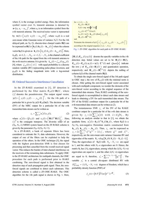
algorithm for the l-th path signal is shown in Fig. 1. Here,
−1
for i = 1, 2, ,
N
F
k l
T
+
ZF, i( l) = Hi( l)
( j)
2
i( ) = arg min fi
( l)
j
( ki
( l))
yk ()( ) ( ) ( )
i l
l = fi l xil
xi+
1
( l) = xi( l) −hk ( )( )
( )( )
i l
l ⋅Quan⎡yk i l
l ⎤
⎣ ⎦
ki
() l
Hi+
1( l) = Hi
( l)
end
T
⎛
⎞
Permutate the elements of y( l) ⎜= ⎡ yk 1() l( l) yk2() l( l) yk ()( )
N l
l ⎤
⎟
R
⎝ ⎣
⎦ ⎠
according to the original sequence ( 1, 2, , NT
).
Fig. 1. ZF-OSIC algorithm for each path in ZF-OSIC-RAKE.
( i(), l
ZF, i(), l
i()
l )
H F x denotes the specific variables in the i-th
detection step. Initial values are set to be H 1
() l = H (), l
( j
FZF,1() l = FZF (), l x1() l = x();
l f ) i
() l and Quan[ i ] indicate
the row j of F ZF, i()( l = H
i() l + ) and quantization operation,
()
respectively; and () k i l
H l H () l depicts the nulling of
i+ 1
=
column k i (l) of the channel matrix H i (l).
To obtain the single zero-forced signal of the l-th path signal
in OSIC step i, the row of F ZF, i (l) with the minimal norm is
chosen. After getting the zero-forced signal vector associated
with each multipath component, we reorder the elements of the
zero-forced vector according to the original sequence of the
transmitted data streams. Then, RAKE combining of the zeroforced
signals is accomplished to detect each data stream and
leads to obtaining a DV for each transmitted data stream. The
DV of the RAKE combiner output for a particular bit of the
n-th transmitted data stream can be written as (2).
The instantaneous SNR γ n
of the DV of the RAKE
combiner output for a particular bit of the n-th data stream is
i
L − 1 2
given by γn
= 2 λ∑ α ( )
l 0 n
l with λ = E
=
s
N0
. By
following an analysis similar to that in [1], we obtain the
quadratic form, α 2 () () H
n
l = hn l Sn() l h
n()
l , where S n (l) is a
N R ×N R non-negative Hermitian matrix constructed from
hn+ 1(), l hn+
2(), l , hN
() l . Then, γ
T
n
can be expressed as
LNR 2
( n) ( n)
γn = 2λ∑ λ
i 1 i
q
= i
= 2λ γ ′
n
, where q ( n)
i
and λ ( n)
i
,
respectively, are the zero-mean unit-variance Gaussian RV and
eigenvalue of the matrix Sn= diag [ Sn(0) Sn(1) Sn( L−1) ].
Thus, the eigenvalues of S n (l) with NR − NT
+ n are equal
to 1, and the others with N T –n eigenvalues are 0. Hence, the
matrix S n has LN R eigenvalues, among which the L(N R –N T +n)
eigenvalues are equal to 1, and the other L(N T –n) eigenvalues
L( NR− N 2
T+
n) ( n)
are equal to 0; therefore, γ ′
n
= ∑ q
i=
0
i
. The
variable γ ′ is a central chi-square distributed RV with
n
( n)
D
ZF-OSIC
=
R T
L( N − N + n)
degrees of freedom, which has a
probability density function (PDF) of
κ
κ−1 −t
2
( κ )
f ′ () t = 0.5 Γ ( ) t e , (3)
γ n
ETRI Journal, Volume 31, Number 4, August 2009 Jinyoung An et al. 473