The Holstein polaron: results from numerical and analytical ... - PiTP
The Holstein polaron: results from numerical and analytical ... - PiTP
The Holstein polaron: results from numerical and analytical ... - PiTP

You also want an ePaper? Increase the reach of your titles
YUMPU automatically turns print PDFs into web optimized ePapers that Google loves.
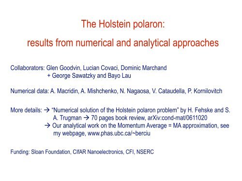
<strong>The</strong> <strong>Holstein</strong> <strong>polaron</strong>:<br />
<strong>results</strong> <strong>from</strong> <strong>numerical</strong> <strong>and</strong> <strong>analytical</strong> approaches<br />
Collaborators: Glen Goodvin, Lucian Covaci, Dominic March<strong>and</strong><br />
+ George Sawatzky <strong>and</strong> Bayo Lau<br />
Numerical data: A. Macridin, A. Mishchenko, N. Nagaosa, V. Cataudella, P. Kornilovitch<br />
More details: “Numerical solution of the <strong>Holstein</strong> <strong>polaron</strong> problem” by H. Fehske <strong>and</strong> S.<br />
A. Trugman 70 pages book review, arXiv:cond-mat/0611020<br />
Our <strong>analytical</strong> work on the Momentum Average = MA approximation, see<br />
my webpage, www.phas.ubc.ca/~berciu<br />
Funding: Sloan Foundation, CIfAR Nanoelectronics, CFI, NSERC
Polaron = electron + lattice distortion (phonon cloud) surrounding it<br />
very old problem: L<strong>and</strong>au, 1933<br />
very many models to study, e.g.<br />
single <strong>polaron</strong> (one extra charge carrier in an insulator) vs. bi-<strong>polaron</strong>s = bound state of two<br />
<strong>polaron</strong>s, vs. many-<strong>polaron</strong>s systems ( metals, superconductors)<br />
large <strong>polaron</strong>s (continous approx) vs. small <strong>polaron</strong>s (lattice model different lattices with d=1,2,3,<br />
different couplings, etc.)<br />
coupling to acoustic or to optical phonon modes, or to both?<br />
<strong>and</strong> then: spin <strong>polaron</strong>s, Jahn-Teller/orbital <strong>polaron</strong>s, …<br />
most famous/studied <strong>polaron</strong> models: Frohlich (continuous model) <strong>and</strong> <strong>Holstein</strong> (lattice model).<br />
Today: review of methods to study the single-<strong>polaron</strong> problem in the <strong>Holstein</strong> model, + some <strong>results</strong><br />
<strong>and</strong> some physics.
Model of interest: the <strong>Holstein</strong> Hamiltonian (1959)<br />
<strong>The</strong> simplest lattice Hamiltonian describing electron-phonon (phonons = lattice vibrations) interactions:<br />
Kinetic energy – describes how<br />
the electron hops on the lattice<br />
Interaction: n i = # of electrons at the site<br />
lattice<br />
Each atom of the lattice is like a harmonic oscillator (quick reminder):<br />
X 0
Hamiltonian was proposed as simplified description of a polar crystal 1D sketch<br />
“unit cell” in<br />
equilibrium<br />
+ δq<br />
- δq<br />
add extra e<br />
= new equilibrium distance<br />
t<br />
<strong>polaron</strong> (small or large, depending) but<br />
always mobile, in absence of disorder<br />
Eigenstates are linear combinations of states with the electron at different sites, surrounded by a<br />
lattice distortion (cloud of phonons).<br />
This composite object = electron dressed by surrounding cloud of phonons is called a <strong>polaron</strong>.
(spin is irrelevant, N = number of unit cells, infinity at the end, all k,q-sums over Brillouin zone)<br />
Asymptotic behavior:<br />
zero-coupling limit, g=0 eigenstates of given k:<br />
with eigenenergies<br />
where, for example,<br />
E k<br />
el + 2 ph continuum<br />
el + 1 ph continuum<br />
Ω<br />
k<br />
single electron
weak coupling, g = “small” low-energy eigenstates of known k:<br />
with eigenenergies (for k< k cross )<br />
E k<br />
<strong>The</strong> phonons can be<br />
quite far spatially <strong>from</strong> the<br />
electron large <strong>polaron</strong><br />
<strong>polaron</strong> + one- phonon<br />
continuum (finite lifetimes)<br />
k<br />
Ω<br />
<strong>polaron</strong> b<strong>and</strong> (infinitely<br />
long-lived quasiparticle)<br />
high-k: wavefunction<br />
dominated by el+1ph<br />
contributions<br />
low-k: wavefunction dominated<br />
by free electron contribution
infinitely strong coupling, t=0 electron stays at a single site forever n i =1 there, 0 elsewhere<br />
→<br />
<strong>polaron</strong> binding energy;<br />
small <strong>polaron</strong> limit<br />
only discrete eigenstates!<br />
Recall coherent states:
Ground-state energy: -2dt (half-b<strong>and</strong>width, at zero coupling) -g 2 /Ω (infinite coupling)<br />
Effective coupling as their ratio λ = g 2 /(2dtΩ) weak coupling λ>1<br />
3 energy scales: t, Ω, g 2 dimensionless parameters λ = g 2 /(2dtΩ), Ω/t (d is lattice dimension)<br />
very strong coupling, λ>>1 <strong>polaron</strong> energy is<br />
Again, must have a <strong>polaron</strong>+one-phonon continuum at E GS + Ω details too nasty<br />
Question: how is the spectrum evolving between these two very different limits?
Quantity of interest: the Green’s function or propagator<br />
eigenenergies <strong>and</strong> eigenfunctions (1 electron, total momentum<br />
k, α is collection of other needed quantum numbers)<br />
A(k,ω)<br />
= spectral weight, is measured (inverse) angleresolved<br />
photoemission spectroscopy (ARPES)<br />
η<br />
Area is equal to Z<br />
Z = quasiparticle weight measures how similar is the true wavefunction to a non-interacting (free<br />
electron, no phonons) wavefunction<br />
ω
weak coupling<br />
Lang-Firsov impurity limit<br />
Ω<br />
How does the spectral weight evolve between these two very different looking limits?
Most <strong>numerical</strong> approaches focus on the evolution of the <strong>polaron</strong> b<strong>and</strong> (low-energy properties)<br />
variational methods (Trugman <strong>and</strong> co-workers)<br />
truncate size of cloud (both spatial <strong>and</strong> how many phonons are allowed) Lanczos<br />
advantages: continuous k (not a finite-size chain!); matrix elements are very simple to get, can be<br />
extremely accurate for discrete states (like the <strong>polaron</strong> b<strong>and</strong> of interest)<br />
disadvantages: at large couplings, very many phonon combinations huge dimension of<br />
variational Hilbert space (gets worse in higher dimension). Also, no predictive powers for the<br />
continuum above the <strong>polaron</strong> b<strong>and</strong> nothing about high-energy properties.
Diagrammatic Quantum Monte Carlo (Prokof’ev, Svistunov <strong>and</strong> co-workers)<br />
calculate Green’s function in imaginary time<br />
Basically, use Metropolis algorithm to sample which diagrams to sum, <strong>and</strong> keep summing<br />
<strong>numerical</strong>ly until convergence is reached<br />
advantages: once code is written, it is fast (min. per data point) <strong>and</strong> very accurate for lowenergies<br />
(discrete eigenstates). In principle it can be used to generate whole G(k,w) but<br />
convergence for short-times is much more difficult, also one needs analytic continuation to switch<br />
to real frequencies A. Mishchenko<br />
disadvantages: writing the code (for me, at least)
Quantum Monte Carlo methods (Kornilovitch in Alex<strong>and</strong>rov group, Hohenadler in Fehske<br />
group, …) write partition function as path integral, use Trotter to discretize it, then evaluate.<br />
Mostly low-energy properties are calculated/shown.<br />
Exact diagonalization = ED finite system (still need to truncate Hilbert space) can get<br />
whole spectrum <strong>and</strong> then build G(k,w)<br />
Cluster perturbation theory: ED finite system, then use perturbation in hopping to “sew” finite<br />
pieces together infinite system.<br />
advantage: can calculate G(k,w) for all k.<br />
disadvantage: problems in higher dimension, <strong>and</strong> lower couplings (big phonon clouds)<br />
“Special” methods:<br />
DMRG (density matrix renormalization group, if d=1)<br />
DMFT (dynamic mean-field theory, if d infinity)<br />
…. (lots of work done in these 50 years, as you may imagine)<br />
<strong>The</strong>y’re all in very good agreement for low-energy properties, the difference is in efficiency<br />
<strong>and</strong> “generalizability” to higher dimensions, other models, etc.
Analytic approaches (other than perturbation theory) calculate self-energy<br />
Σ(k,ω) = + + +….<br />
For <strong>Holstein</strong> <strong>polaron</strong>, we need to sum to orders well above g 2 /Ω 2 to get convergence.<br />
n 1 2 3 4 5 6 7 8<br />
Σ, exact 1 2 10 74 706 8162 110410 1708394<br />
Σ, SCBA 1 1 2 5 14 42 132 429<br />
Traditional approach: find a subclass of diagrams that can be summed, ignore the rest<br />
self-consistent Born approximation (SCBA) – sums only non-crossed diagrams (much fewer)
New proposal: the MA (n) hierarchy of approximations:<br />
Idea: keep ALL self-energy diagrams, but approximate each such that the summation can be<br />
carried out <strong>analytical</strong>ly. (Alternative explanation: generate the infinite hierarchy of coupled<br />
equations of motion for the propagator, keep all of them instead of factorizing <strong>and</strong> truncating, but<br />
simplify coefficients so that an <strong>analytical</strong> solution can be found).<br />
First: MA (0) – simplest (least accurate) version<br />
Replace each<br />
in the self-energy diagrams by<br />
one can sum all the resulting self-energy diagrams:<br />
result is EXACT both for g=0 <strong>and</strong> for t=0<br />
trivial to evaluate<br />
<strong>The</strong>re are good reasons why this should work well at low energies (ask!)<br />
This approx. obeys exactly multiple sum rules for the spectral weight (at least 6)
2D <strong>results</strong> for ground-state properties
3D Polaron dispersion<br />
L. -C. Ku, S. A. Trugman <strong>and</strong> S. Bonca, Phys. Rev. B 65, 174306 (2002).
λ = 0.5 λ = 1<br />
λ = 2<br />
A(k,ω) in 1D, Ω =0.4 t<br />
G. De Filippis et al, PRB 72, 014307 (2005)<br />
MA becomes exact for small, large λ
MA (0) is remarkably good, especially considering how simple it is. Higher d is equally trivial<br />
as d=1. However, it is an approximation, <strong>and</strong> it does have its problems:<br />
self-energy is momentum independent<br />
the accuracy worsens if Ω/t 0<br />
doesn’t see the <strong>polaron</strong>+one phonon continuum where it should be<br />
E GS + Ω – continuum must always start above this energy<br />
1D, Ω =0.5t, λ =0.25
Problems easy to fix improve the approximation:<br />
MA (n) keep free propagators of frequency ω – mΩ, m < n exactly in the self-energy<br />
diagrams; all propagators with more phonons (lower energy) are momentum averaged<br />
MA (1) – G 0 (k-q,ω−Ω) contributions exact, lines with 2 or more phonons are momentum<br />
averaged.<br />
MA (2) – G 0 (k-q,ω−Ω), G 0 (k-q,ω−2Ω) contributions exact, lines with 3 or more phonons<br />
are momentum averaged, etc.<br />
Still can sum all diagrams in the self-energy, calculation still <strong>numerical</strong>ly trivial
details in PRB 76, 165109 (2007)<br />
(models with g(q) coupling have a k-dependent self-energy <strong>from</strong> level MA (0) )
1D, Ω=0.5t<br />
1D, Ω=0.1t<br />
λ = 0.6<br />
λ = 1.1<br />
Sum rules:<br />
MA (0) exact up to n=5 <strong>and</strong> accurate above; MA (1) exact up to n=7 <strong>and</strong> more accurate<br />
above; MA (2) exact up to n=9 <strong>and</strong> yet more accurate above, …
1D, Ω =0.5t, λ =0.25
1D, k=0, Ω=0.5t<br />
MA (0) MA (2)
Our answer to how spectral weight evolves as λ increases <strong>from</strong> weak to strong coupling
Generalizations:<br />
Lucian: multiple phonon modes <strong>and</strong>/or multiple free-electron b<strong>and</strong>s (but <strong>Holstein</strong> coupling)<br />
Glen: el-ph coupling which depends on phonon momentum<br />
Example: coupling to breathing-mode phonon (phonons live on different sublattice than the electron)<br />
bi<strong>polaron</strong>s (well advanced)<br />
future: finite-T, other quantities (optical<br />
conductivity), higher concentrations, models<br />
with g(k,q), ….<br />
Numerics: Bayo Lau, M. Berciu <strong>and</strong> G. A. Sawatzky, PRB 76, 174305 (2007)
Why should this be a reasonable thing to do?<br />
(i) Real-space argument: MA (0) means<br />
i<br />
j<br />
i<br />
j<br />
At low energies ω ~ E GS < -2dt free electron Greens’ functions decrease exponentially<br />
with distance |i-j| MA (0) keeps the most important (diagonal) contribution. <strong>The</strong><br />
approximation becomes better the more phonons are present, since the lower ω – n Ω is,<br />
the faster the decay.<br />
Expect ground-state properties to be described quite accurately.
(ii) Spectral weight sum rules (see PRB 74, 245104 (2006) for details)<br />
can be calculated exactly<br />
MA (0) satisfies exactly the first 6 sum rules, <strong>and</strong> with good accuracy all the higher ones.<br />
Note: it is not enough to only satisfy a few sum rules, even if exactly. ALL must be satisfied as well<br />
as possible.<br />
Examples: 1. SCBA satisfies exactly the first 4 sum rules, but is very wrong for higher order sum<br />
rules fails miserably to predict strong coupling behavior (proof coming up in a minute).<br />
2. Compare these two spectral weights:<br />
-w 0<br />
0 w 0
Since G(k,w) is a sum of diagrams, keeping the correct no. of diagrams is extremely important!<br />
found correctly if n=0 diagram kept correctly dominates if t >> g, λ 0<br />
found correctly if we sum correct no. of<br />
diagrams dominates if g >>t, λ >>1