Voxels in ASAP - Breault Research Organization, Inc.

ASAP TECHNICAL PUBLICATION 

BROPN1158 (MARCH 20, 2008) 

Voxels in ASAP 

Modeling fluorescence and volume scatter 

This technical publication describes a powerful ASAP command, VOXELS, in the Advanced Systems Analysis 

Program (ASAP®) from Breault Research Organization (BRO). The VOXELS command in ASAP studies the 

flow of energy in an arbitrary volume in space. It expands our ability to model many optical effects previously 

inaccessible. Energy flow is detected by either using three-dimensional elements, called voxels, 

or by multiple irradiance detectors along a selected axis. Which method is chosen depends on the user 

application and a clear understanding of how the VOXELS command works. This technical publication 

concentrates on the use of VOXELS for modeling fluorescence, and for studying the effects of another 

ASAP feature, volume scatter. 

Green rays are created 

from absorbed red rays 

(some rays were not 

plotted. 

Short low-level 

Total output with 

leakage 

fluorescence 

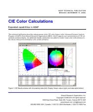
Figure 1 Fluorescence in transmission, by re-emission of radiation that is absorbed in a voxel volume 

Breault Research Organization, Inc. 

Copyright © 2006-2014 All rights reserved. 

6400 East Grant Road, Suite 350, Tucson, Arizona 85715 USA 

www.breault.com | info@breault.com 

800-882-5085 USA | Canada | 1-520-721-0500 Worldwide | 1-520-721-9630 Fax


Fluorescence is generally described as the spontaneous emission of light by a substance at a longer wavelength, 

due to absorption of radiation at a shorter wavelength. To model this, we need to supply ASAP with the exact 

properties of the fluorescent material, such as its absorption and quantum efficiency. 

Volume scatter allows us to simulate additional effects inside a source, or any other translucent scattering material. 

A voxel could be described as a 3D pixel. The major advantage it has over its two-dimensional (2D) counterpart 

is that it can measure the amount of energy passing through its 3D borders from any direction. Each voxel represents 

an individual element of a larger 3D array, defining a region of space in which we want to measure the 

flow of energy. Each voxel will be assigned a single value representing flux-per-unit-volume. The size of these 

voxel elements is determined by the extents of the region in all three coordinate axes, and the resolution for each. 

VOXELS command 

With the VOXELS command, we can capture the absorbed energy as we trace through a volume that physically 

matches the material dimensions. A three-dimensional (3D) data file is created, representing the distribution of 

flux throughout this volume. This distribution data can be easily turned into a new source at a new wavelength, 

using commands in ASAP. 

ASAP offers a choice of three modifiers to the VOXELS command, depending on the application. In this section, 

we will study the processes behind these options and consequences for each, to make an informed decision. Note 

that only two of these modifiers can be used to set up an array of voxel elements, as the name implies, ABSORBED 

and FLUENCE. See Figure 2. 

Figure 2 Voxel elements using ABSORBED or FLUENCE 

A voxel element can be described as a 3D pixel. Its major advantage over its two-dimensional (2D) counterpart 

is that it can measure the energy of rays passing through its 3D borders from any direction. A single value located 

at the center of the voxel represents the total flux of all these rays in flux/units-cubed. The voxel is part of a larger 

3D array, defining a region of space in which we want to measure the flow of energy. The size of the voxel is 

determined by the extents of the region in all three coordinate axes, and the resolution for each. 

2 Voxels in ASAP

. . . . . 

Using real ray path information, or OPL of the ray, ASAP determines whether it has intersected a voxel from any 

direction. It then adds this flux contribution or absorption to the voxel total. The FLUENCE option was initially 

designed for high-energy applications, where the flux density through a laser cavity medium was to be analyzed. 

With voxels, it is important to understand that an equal amount of flux gets recorded whether it passes 

straight through the voxel or grazes it at an angle across the corner. There is no adjustment of flux based 

on angle or amount of the volume traversed. 

CAUTION When dealing with a diverging or converging grid of rays, an over-estimation of flux can easily 

occur. We can see this effect of over-estimation of flux in Figure 3 where the FLUENCE modifier was used 

to capture flux from two converging rays. Using a starting flux of 1 for each ray, the total flux in each 

voxel is recorded in red. 

Figure 3 Flux contribution using voxels 

This method of recording flux can cause clumping in the data distribution, similar to standing waves 

or super-position of beams in coherent work. Increasing the number of voxels and rays will improve 

results, but this sampling effect may still remain, though to a lesser degree. For best performance, 

ABSORBED or FLUENCE should be used only with random emitting sources, or for analyzing scattered 

rays. The 3D Viewer comparison in Figure 4 shows smoother results can be achieved with random rays 

Voxels in ASAP 3


for the same converging cone. 

Figure 4 BRO 3D Viewer showing data clumping using voxels with a grid (left) versus smoother results obtained 

with random rays (right) 


. . . . . 

For the third option on the VOXELS command, an axial modifier (X, Y, Z) tells ASAP to capture flux/ 

units-squared on irradiance planes at equal intervals. See Figure 5. 

Figure 5 VOXELS using axial analysis 



This method does not suffer the sampling effects noted in and therefore gives a smoother 3D distribution, with 

the correct flux calculated from plane to plane. In Figure 6, we see that the same two rays each get counted only 

once as they pass through each pixel. No clumping can occur here. 

Figure 6 Flux contribution using pixels 

However, even with this method, drop-outs or aliasing can occur from rays skipping every other pixel at certain 

angles, especially with converging/diverging grid sources. This general sampling issue can be minimized by using 

plenty of rays with enough pixels and slices to adequately sample the narrowest portion of the beam. 

Whichever form of the command is chosen, the VOXELS region must always be defined before a ray trace is performed. 

The volume data is then captured in a special 3D distribution file during the trace. This region may be 

located anywhere in the system, but is usually matched to a specific object of interest containing some unusual 

medium. In this way, only the energy of rays traced though this medium is captured. 

NOTE Rays must be traced to real surfaces on the far side of the volume or they will not be recorded. In 

other words, they need to be “going somewhere”. Typically, all sides of the volume are enclosed by 

surfaces. 

Two methods exist for setting up the extents of the capture region and resolution in all three dimensions: 

1 The “short form” uses the prior WINDOW and PIXELS settings to tell ASAP the lateral extents and 

resolution of the region. You need to supply only the start and end positions along the coordinate 

axis (perpendicular to the window), and the corresponding number of steps or slices, along that 

direction. These “slices” can be extracted as separate display files. They are either slices 

through the middle of a plane of voxels, or an irradiance slice, depending on options used. 

2 The “long form” is a more direct approach, which allows specifying all parameters of the volume 

in the Command Input window at once, with no regard to WINDOW or PIXELS. In this case, the 

slices are always stored along the Z axis. 


. . . . . 

Using VOXELS for capturing fluence 

As an example, the VOXELS command can be used to describe a particular volume surrounding a medium in 

which a particular volume scatter function is applied. Using VOXELS with the axis modifier allows us to capture 

and analyze the effects of this scatter through the volume. This is best studied in the 3D Viewer as shown in Figure 

7. 

Figure 7 Raytrace in a scattering medium captured with VOXELS Z 

The following command script was used to capture the flux-per-unit-area as it passed through 100 slices in the 

Z direction for that figure: 

VOXELS Z -1 1 -1 1 4 50 50 100 

The axial modifier tells ASAP to capture the flux-per-unit area, either unidirectionally or bidirectionally, in irradiance 

slices, along the specified coordinate axis. In this case, “Z” does not give preference to any direction, 

as opposed to +Z or Z. Therefore, the total flux within the volume may rise above what we started with, though 

the flux exiting the volume will be correct. For incoherent scatter analysis, we may want to single out a particular 

direction to maintain flux conservation. Due to the nature of using irradiance planes, a small portion of rays can 

escape out the sides of the volume. These can be captured by detectors, but the effect becomes insignificant as 

more planes are specified and the spacing narrows. 

NOTE Similar results to above, at least visually, can be achieved using the FLUENCE modifier, rather than 

by axial direction. FLUENCE will record the total flux passing through each voxel in any direction with no 

concern about lost rays. Sampling issues due to flux clumping will still exist, but not as much of an 

issue with random scatter rays. It is still recommended to use enough voxels and rays to minimize 

errors in flux calculation. 

Using VOXELS to capture absorbed energy 

Since the axial modifier (without the sign) allows capturing flux bi-directionally, nothing prevents us from using 

it with absorbing media, though we would need to calculate the total absorbed flux manually. Of course, this may 

not be a problem for single or multiple passes through the volume from one end to another. However, for the case 

when rays are coming through from all sides, or with volume scattering, it would be almost impossible to calcu- 



late total absorption unless the ABSORBED modifier was used. Again, we must use enough slices and voxels to 

improve flux calculation. The following example script uses the long-form version of the command: 

VOXELS ABSORBED -1 1 -1 1 1 4 51 51 200 

This script produces the image in Figure 8 of a converging grid of incoherent rays. 

Figure 8 Voxel distribution of absorbed energy, using the keyword ABSORBED 

ABSORBED tells ASAP to capture the energy that was lost to absorption within the volume. For this case, the defined 

region was matched to a medium with a complex index of refraction. During the trace, the total energy 

absorbed from rays passing through this region was recorded for each of the voxel elements. Absorption is omnidirectional 

by nature, so no option is needed to make it directional. Clicking a plane in the 3D Viewer shows 

the flux per unit volume at the center of that voxel. The Command Output window will report the Total flux absorbed 

in VOXELS, though this may be overestimated if not enough voxels were used. 

In the case shown here, we purposely used a non-random grid of converging rays to show the hotspots and dropouts, 

especially with such a low number of voxels. For certain simulations, ABSORBED may be the only option, 

but for a single-pass non-scattering system like this, a smoother more accurate distribution can be achieved using 

the axial modifier, as such: 

VOXELS Z -1 1 -1 1 1 4 51 51 200 

In this case, no “total absorption” is reported in the Command Output window. However, we can do this calculation 

easily by measuring the output flux residing on surfaces at the far end of the volume. This can be used later 

to normalize a new source created from this distribution. 

VOXELS command syntax and accessing data 

So far, we have been using the long form of the VOXELS command. The first six numbers represent the limits of 

the volume in x, y, and z. These should be matched to the volume you want to measure in the geometry. The 

other numbers describe the lateral extent in pixels and slices in the axial direction as shown in the previous pictures. 

Currently, only rectangular volumes are possible with VOXELS. 


. . . . . 

The 3D array of data from VOXELS is automatically saved during the ray trace to a special temporary file, 

BRO009.DAT. This data may be stored under a permanent file name using the WRITE command. The distribution 

is a multi-dimensional display file containing individual “irradiance” slices (or volume slices using FLUENCE 

or ABSORBED), which are always stored along the coordinate axis (assumed to be the Z axis when using the long 

form of the command). However, as we see in previous figures, we can always view the 3D data in real time in 

any direction by simply opening the data file directly in 3D Viewer. It helps if we have already plotted the geometry 

so it can be partially displayed as reference. 

When viewing 3D data files, ASAP supplies two planes in each axis, which may be moved forward or backward 

to study individual planes from any view angle. Some planes were removed from these pictures for clarity. (For 

those who use coherent ASAP, this process may look familiar, as it is the same method used for many years to 

view multiple-plane FIELD files.) 

To perform 2D display analysis (such PICTURE, GRAPH, or CONTOUR), we use DISPLAY, followed by the file 

name (or use “9” for the default file bro009.dat) and the “slice” number. In our previous example using 

ABSORBED, 200 slices were stored along the Z axis. 

Figure 9 shows slice 100 of the 200 total slices in Z. We have included two results, as another way to view the 

flux clumping in voxels when using a uniform grid, as opposed to a random emitter. 

Figure 9 PICTURE comparing slice 100 with converging GRID (left) versus converging EMITTER (right) 

NOTE The numbering of slices always increases in the direction of propagation. If no number is specified 

with DISPLAY, the last slice in the volume is accessed by default. 

These slices are the same as the planes viewed in the 3D Viewer along the coordinate axis. They are centered on 

the pixels or voxels in that direction. For example, if we ask for 10 slices between Z=20 and Z=30, the first slice 

will be at 20.5 (for DISPLAY 9 1) and the last slice at 29.5 (for DISPLAY 9 10). This is because ASAP always 

divides up pixels within the range specified, not including end points. The Command Output window reports the 



Z position, which should match that obtained by clicking in the 3D Viewer. For voxel slices, these planes actually 

cut through the center of the voxels. For irradiance slices, these planes are at those fixed positions. 

If you need to extract slices in a direction orthogonal to the normal coordinate axis, use the short form of VOXELS. 

This way, slices are stored in the given depth range that is perpendicular to the last WINDOW setting. The previous 

PIXELS command is used to determine the resolution in the orthogonal directions. 

NOTE ASAP can not record flux through more than one voxel volume at a time during a trace. Of course, 

this includes overlapping volumes. If slices are to be extracted for each direction separately, a new 

TRACE is required for each. Optionally, the capturing of flux through the VOXELS volume may be turned 

OFF or ON as needed during tracing. 

Modeling fluorescence: creating a new source from stored distribution data 

Now that we can store a 3D display file using the VOXELS command, we can turn it into an emitting source simply 

by using the EMITTING DATA command in our ASAP script. This is the same powerful command we have 

always used in ASAP to create sources from saved display or ray files. If we want to change the wavelength, as 

with a fluorescent source, we first issue a new WAVELENGTH command. Generally, this has a longer wavelength 

than the one used in the first trace and an associated media index with little or no absorption. Assuming the 

VOXELS distribution file was saved under the name “ABS_FLUX”, an example of a command line for creating 

a new source is: 

EMITTING DATA ABS_FLUX 100000 

This script generates 100K rays randomly and isotropically from the volume data stored in the file. Its distribution 

may be adjusted, if needed, by the usual ASAP commands, such as CLIP (directional cone of radiation) or 

USERAPOD (angular apodization of flux). Either CLIP or the SELECT ONLY command can be used to specify a 

positive or negative direction down the propagation axis. This approach can be useful to simulate fluorescence 

in reflection or transmission, and save raytrace time. CLIP is used before EMITTING DATA, to create only those 

rays in the desired direction. Typically, the emitting source follows the rectangular shape of the initial voxels 

volume. If desired, we can use the BOUNDS command to trim the source to some other arbitrary shape. This subject 

is covered in another ASAP technical publication, Arrays and Bounds. This and other BRO technical publication 

referenced in this document may be viewed or downloaded from the BRO Knowledge Base, 

http://www.breault.com/k-base.php. 


. . . . . 

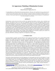
Figure 10 shows a simplified example that clearly demonstrates absorption along a volume, overlaid with the 

new source. Geometry is drawn to help visualize the beginning and end of the volume. The spots show the initial 

ray-density distribution of the new source, based on absorption data. 

Figure 10 Absorption turned into a new source 

A generic ASAP script may look like Figure 11. 



SYSTEM NEW 

RESET 

UNITS MM 

WAVELENGTHS 450 633 NM !! Wavelength range 

MEDIA 

1.5` .4E-4 1.2 'TEST' !! Absorb at 450nm 

FRESNEL TIR 

!! Rays will TIR towards edges 

CEFF-.60 

!! Conv. eff. of fluorescent mat'l 

***GEOMETRY GOES HERE*** 

WAVELENGTH 450 NM 

EMITTING DISK Z 0 2@1 8000 0 0 !! Source 

FLUX TOTAL 100.0 

!! Set initial flux 

VOXELS ABSORBED -4@1.2 1 4 50 50 100 

WINDOW Y Z 

PLOT FACETS COLOR 2 OVERLAY 

TRACE PLOT OVERLAY 

$GRAB 'VOXELS' F_ABS !! Grab absorbed flux 

$COPY 9 ABS_FLUX.DIS !! Copy default file to ABSORB.dis 

RAYS 0 

!! Clear out previous rays 

WAVELENGTH 633 NM !! Change wavelength 

IMMERSE TEST 

!! Start new source in media 

CLIP DIR -1 1 -1 1 0 1 !! Create +Z rays 

EMITTING DATA ABS_FLUX 100000 !! New source 

FLUX TOTAL F_ABS*CEFF !! Fluorescent flux 

SPOTS POSITION OVERLAY !! Show new source spots 

VOXELS OFF 

!! Turn off voxel data capture 

TRACE PLOT 

!! Trace new source 

***MORE ANALYSIS GOES HERE*** 

$VIEW 

!! Show in 3D Viewer 

&VIEW ABS_FLUX.DIS !! Add absorption distribution 

RETURN 

Figure 11 Simplified ASAP script to create fluorescence from absorption 

The script in Figure 11 is similar to what might be used to model fluorescence in transmission, as shown in Figure 

1. Note the original rays are cleared out with a RAYS 0 command before the new emission source is traced. The 

total flux of the new source will not need adjustment if the ABSORBED modifier were used to create the distribu- 


. . . . . 

tion initially. If it were created using an axial modifier instead, the flux should be normalized according to the 

calculated absorption. 

Figure 12 shows a model of fluorescence in reflection. To trace the new source in the reverse direction, we again 

use CLIP to create only those rays needed. For this particular example, a diffuser screen is placed just above the 

fluorescing material, which uses the technique of scattering towards an importance edge. This directs the rays 

more efficiently through the microscope optics. 

Figure 12 Fluorescence in reflection through a microscope 

Whether we trace rays in reflection or transmission, the IMMERSE command is used to specify the MEDIA where 

the new rays are created by the EMITTING DATA command. These rays are considered to be inside the fluorescent 

media, instead of in air (the default). Depending on the index relative to air at the excitation wavelength, a 



certain amount of flux is lost due to total internal reflection (TIR) of higher-angle rays. The TIR is absorbed at 

the edges of the material. 

We do not need to limit the EMITTING DATA command to using a volume source for simulating fluorescence. 

A simpler option exists for those who need only an infinitely thin material to fluoresce. This option could be a 

single plane, where an irradiance distribution is created with a SPOTS POSITION command. The resulting display 

file is easily turned into a new 2D source using EMITTING DATA in the same way as the volume source. 

The main difference is that the radiation is Lambertian and its direction can be controlled with a or + before 

the DATA keyword. The appropriate flux may be assigned to the new source, and it can also be apodized in direction 

or position. 

Real-world considerations 

Typically, an accurately designed fluorescence simulation could become quite elaborate. We may want to model 

the fluorescent emission from the substance, but also account for original source flux that is transmitted through 

the material or scattered from adjacent surfaces. To do this, we can let the original raytrace reach the detector, 

make a spots distribution, and then add the second distribution from the fluorescence trace, using the COMBINE 

command. This command allows the summing together of distribution files having the same WINDOW area 

PIXELS resolution. The example shown in Figure 1 uses this technique. 

We can turn on or off the accumulation of data by the VOXELS command, allowing us to add up irradiance 

through a volume over several traces. This accumulation might be valuable when there is more than one source 

involved, and these sources need to be traced separately. 

We can now collect data from absorption, scatter, or both in a VOXELS distribution file, and then turn it into a 

new source, if we want. Absorption, modeled by assigning a complex index of refraction, or an absorption coefficient 

(per unit length), is a way of describing how a ray’s flux changes as it travels a distance through a medium, 

and is a standard concept in ASAP. Volume scatter is relatively newer, and is a bit more involved. 

Therefore, to complete our discussion of fluorescence modeling and volume analysis, we will take a closer look 

at the details of volume scatter in ASAP. 

Modeling volume scatter 

Volume scatter is just another way to describe an ASAP medium in which rays are affected as they travel through 

a length of that medium. Rather than a change in flux or an index variation (MEDIA...GRIN), volume scatter 

directly affects ray directions. Undoubtedly, there are applications that exist that require a source based on volume 

scatter, or one that must integrate it in some way. 

An example might be studying near-field effects of rays interacting with a plasma. These rays may be reflected 

back through a clear envelope from a reflector nearby, which changes the source’s pattern. Of course, this is best 

avoided by careful design of the reflector. However, if we must study the effects, we would require some advance 

knowledge of the complex nature of the plasma. This data must be converted into a volume scatter model, possibly 

combined with absorption. Even when modeling a standard fluorescent material, there will probably be a 

need to model its scattering properties, along with its absorption. 

In ASAP, two commonly used methods exist for setting up a volume scatter medium. The first is a carryover 

from a 2D surface scatter model in ASAP—the MIE particles model, where random scattering spheres are distributed 

throughout a volume. The refractive index for the bulk of the scattering medium must be specified, as 

well as the index for the scattering particles (spheres). The five steps to this particular model in ASAP are: 


. . . . . 

1 Specify the MEDIA index for the particles. 

2 Specify the MEDIA index for the bulk volume. 

3 IMMERSE into the volume media, needed to calculate the MIE scatter function next. 

4 Set up the volume scattering MODEL, referencing the particle index (in step 1) for the particles. 

The particle radii range can either be given in fractional wavelength units or directly in 

wavelength units. They become immersed in the bulk media. 

5 Specify MEDIA again, making sure index matches exactly to the bulk volume index above. 

Reference the volume scattering model from step 4. Give this a unique name for use on the INTERFACE of the 

scatter volume boundary surfaces. 

An ASAP script might look like Figure 13. 

Figure 13 Volume scatter: example of method 1 

The PLOT option may be applied to the MODEL in Figure 13 to show the calculated results in ASAP, 

using MIE theory. 

NOTE For good plot resolution, specify beforehand PIXELS 501 or higher. Also, when using volume 

scatter, always set the scatter LEVEL to a very high value (for example, 1000). 

An absorption may be applied to the volume media by specifying a complex index of refraction. Confirm 

that this number is identical for both the bulk media under the first MEDIA statement and the scatter 

volume under the last MEDIA statement. 

ASAP performs an exact calculation based on all data provided. Typically, scattering media is isotropic due to 

the random nature of the molecules in the path. However, for those special cases where the scatter may be nonuniform, 

an option to “MEDIA;SCATTER” can reference a USERFUNC surface, or FORTRAN USER function, 

to specify inhomogenous particle size distribution. There is also a faster MIE approximation—the VOL- 

UME MIE command—using only two parameters, when the spheres are basically opaque (indices>>1), and their 

sizes are large compared to a wavelength. See online Help in ASAP for more information. 



The second method for volume scattering is a more straightforward Monte-Carlo scatter using the Henyey- 

Greenstein model, as shown in Figure 10. 

Scatter 

direction 

Scatter efficiency 

per particle 

Fractional 

obscuration 

Figure 14 Volume scatter: example of method 2 

The first parameter (scatter direction) may range from perfect backscatter (-1), to perfect forward scatter (1), 

where 0 is purely isotropic. The second parameter (scatter efficiency) can also have attached to it another argument 

to provide absorption efficiency (for example, 0.8‘0.2, for 80% scatter and 20% absorption). 

For whichever scatter method is used, the “fractional obscuration” can be found from the particle density in the 

volume (1/mm 3 ), and the cross-sectional area of the particle (mm 2 ). The product of these two is the number to 

use here. It is essentially the inverse mean-free path, or how far the average ray travels in the volume before making 

a turn. 

Figure 15 shows an example of the second method used inside a slab with a Gaussian roughness applied to the 

side walls. With all the options for volume and surface scatter in ASAP, the possibilities seem endless. 

Figure 15 Scatter media with rough walls 


. . . . . 

NOTE For the sake of completeness, there is a third option for defining a scatter medium—MEDIA; 

USER—which calls the USERSCAT function contained in the userprog.dll. You may modify this function 

to allow wavelength change at the media interface. This function can be useful in fluorescence or Raman 

scattering applications. USERSCAT is one of several functions that may be modified using the 

FORTRAN source file, userprog.f90 (ASAPxx\src folder). Further discussion goes beyond the scope of 

this document. Search in online Help in ASAP under “userprog.dll” for more details. 

Summary 

We have two choices when it comes to storing energy traversed throughout a 3D volume of space. One is to record 

the fluence or absorption by using individual 3D elements called voxels. They may be set up in any size or 

number to suit the region of interest and resolution required. Usually, this region is matched to a particular medium 

having specific properties of absorption or scatter that we want to analyze. 

The second choice is to record fluence by a series of irradiance slices along a specific propagation direction or 

axis. This method is generally more accurate for focused non-random rays, or when lower volume resolution is 

used. 

Volume data is stored during the ray trace as a multi-dimensional file, which supports a variety of options for 

analysis. The file is arranged in slices along the specified depth in the coordinate axis. For voxels, the pixels in 

each slice represent flux-per-unit-volume. For “irradiance” slices, the pixels are measured in flux-per-unit-area. 

The BRO 3D Viewer is particularly useful for displaying these volume files. 

Using the same principle available in ASAP to turn a 2D distribution into an emitting source, we can now convert 

a volume distribution of absorption data into a new source, assigning it a new wavelength. This allows us to model 

a fluorescent source that has some thickness or 3D quality. We can limit the direction of this new source and 

apply special angular qualities, as required. Since ASAP has the flexibility of tracking any effects we want to 

ascribe to a volume region, the model may include additional effects, such as from volume scatter or scatter from 

surrounding surfaces. 

Volume scatter is applied as part of the MEDIA command, and is done in two ways. One method uses a more 

well-known but complicated MIE particle model and the other uses a simpler Henyey-Greenstein model. Both 

include the option of adding absorption. Using the particle model, we can apply a complex refractive index to 

the volume medium itself, similar to when we set up absorption alone. In the second model, we can specify absorption 

efficiency as an option added to scatter efficiency. 

Whatever effects we want to simulate inside a volume, whether it is for creating a new fluorescent source, or 

studying a type of translucent scattering material, we have the VOXELS command to help us. As with any simulation, 

the accuracy of the results depends highly on the quality of the data we use to model it, and the knowledge 

of the tools that ASAP makes available.

Voxels in ASAP - Breault Research Organization, Inc.

You also want an ePaper? Increase the reach of your titles

Delete template?

Save as template?