SOURCES IN ASAP - Breault Research Organization, Inc.
SOURCES IN ASAP - Breault Research Organization, Inc.
SOURCES IN ASAP - Breault Research Organization, Inc.

Create successful ePaper yourself
Turn your PDF publications into a flip-book with our unique Google optimized e-Paper software.
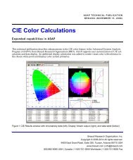
<strong>ASAP</strong>. . . . . . . . . . . . . . . . . . . . . . . . . . . . . . . . . . .. . . . .Technical Guide<strong>SOURCES</strong> <strong>IN</strong> <strong>ASAP</strong><strong>Breault</strong> <strong>Research</strong> <strong>Organization</strong>, <strong>Inc</strong>.
. . . . .This Technical Guide is for use with <strong>ASAP</strong>®.Comments on this manual are welcome at: support@breault.comFor technical support or information about other BRO products, contact:US/Canada: 1-800-882-5085Outside US/Canada: +1-520-721-0500Fax: +1-520-721-9630E-Mail:Technical Customer Service:support@breault.comGeneral Information:info@breault.comWeb Site:http://www.breault.com<strong>Breault</strong> <strong>Research</strong> <strong>Organization</strong>, <strong>Inc</strong>., (BRO) provides this document as is without warranty of any kind, eitherexpress or implied, including, but not limited to, the implied warranty of merchantability or fitness for a particularpurpose. Some states do not allow a disclaimer of express or implied warranties in certain transactions;therefore, this statement may not apply to you. Information in this document is subject to change without notice.Copyright © 2003-2013 <strong>Breault</strong> <strong>Research</strong> Corporation, <strong>Inc</strong>. All rights reserved.This product and related documentation are protected by copyright and are distributed under licenses restrictingtheir use, copying, distribution, and decompilation. No part of this product or related documentation may bereproduced in any form by any means without prior written authorization of <strong>Breault</strong> <strong>Research</strong> <strong>Organization</strong>, <strong>Inc</strong>.,and its licensors, if any. Diversion contrary to United States law is prohibited.<strong>ASAP</strong> is a registered trademark of <strong>Breault</strong> <strong>Research</strong> <strong>Organization</strong>, <strong>Inc</strong>.<strong>Breault</strong> <strong>Research</strong> <strong>Organization</strong>, <strong>Inc</strong>.6400 East Grant Road, Suite 350Tucson, AZ 85715brotg0911_sources (November 13, 2008)<strong>ASAP</strong> Technical Guide 3
Contents. . . . . . . . . . . . . . . . . . . . . . . . . . . . . . . . . . .. . . . .Sources in <strong>ASAP</strong> 7One ray at a time 8BRO Light Source Library 9Radiant Imaging sources 12CAD-imported objects as EMITT<strong>IN</strong>G OBJECTs 12Saving and recalling rays 13Saving and Recalling Rays using DUMP and EMIT DATA 14Emitting Bitmaps 16Source apodization 17Immersing sources 24IMMERSE Command 24Multiple wavelengths 25Creating multi-color sources within <strong>ASAP</strong> with SPECTRUM 28Setting the flux 33Review 34<strong>ASAP</strong> Technical Guide 5
<strong>SOURCES</strong> <strong>IN</strong> <strong>ASAP</strong>. . . . . . . . . . . . . . . . . . . . . . . . . . . . . . . . . . .. . . . .In Chapters 7, 8, 9,10, 11, and 16 of the <strong>ASAP</strong> Primer, we covered most of the basicinformation about creating sources in the Advanced Systems Analysis Program (<strong>ASAP</strong>®)from <strong>Breault</strong> <strong>Research</strong> <strong>Organization</strong> (BRO®), and discussed, to some degree, how theycould be manipulated in space and in magnitude. We learned how to create two-dimensionalgrids and surface emitters, apply directionality to the rays, and position them in space. Wealso looked at how to make volume emitters from general, three-dimensional shapes.In this technical guide, we apply some new techniques to these sources and introduce somealternative sources as well. We also cover some specialty topics and discuss multiplesources and wavelengths. This technical guide addresses the following topics:1 How to input rays one at a timeInputting rays is useful when you know the exact location and direction of the rays youwant, or have a large file of rays to import.2 Using the BRO Light Source LibraryThe BRO Light Source Library, available to <strong>ASAP</strong> customers with current softwaremaintenance agreements, is a growing collection of more than 150 U.S. and Europeansource models that can be imported directly into <strong>ASAP</strong> projects. The library includesfilament, light-emitting diode (LED), arc, and cold cathode fluorescent (CCF) sources.These sources include detailed geometry and produce near- and far-field patterns that are inagreement with measurements. We will show you how easy it is to use, and the variousways you can use it.3 Using Radiant SourcesThese are source files created by Radiant Imaging, <strong>Inc</strong>. for a special source you may need toanalyze in your system. The distribution file should be obtained from Radiant Imaging(http://www.radimg.com/) in the <strong>ASAP</strong> format for distribution files.4 EMITT<strong>IN</strong>G OBJECT using CAD-imported objectsAny object in <strong>ASAP</strong>, including objects imported from a CAD program, can be made into asurface emitter with the EMITT<strong>IN</strong>G OBJECT command.5 Saving and recalling raysWe will show you how to use the DUMP command to save rays at any point in your system,and how EMITT<strong>IN</strong>G DATA can bring them back. You will see how this was done in theLight Source Library.6 Apodizing sources with USERAPOD or APODIZE<strong>ASAP</strong> Technical Guide 7
<strong>SOURCES</strong> <strong>IN</strong> <strong>ASAP</strong>Apodizing in <strong>ASAP</strong> means making changes in the spatial or angular distribution of the raysfrom a source. This is accomplished by applying your own measured data or a function,using several approaches that are available. We will discuss each of these and giveexamples.7 Originating sources in a mediumSince the default medium in <strong>ASAP</strong> is VACUUM/AIR, it is also assumed that the rays of asource will begin there as well. However, an application such as an LED source may requiresomething different. We will show you how to change the medium where the rays begin.8 Multiple sources and multiple wavelengthsYou need to understand how to set up multiple sources at different wavelengths, so that<strong>ASAP</strong> makes the proper refraction or Fresnel calculations in your model.9 Controlling the flux with the command languageWhen setting the flux of multiple sources, there are certain things to be aware of. We willdiscuss the FLUX command in combination with SELECT ONLY, and show how to changethe default name for the units of the radiant power.One ray at a time<strong>ASAP</strong> offers two methods for entering individual rays. Each has its particular uses,depending on the application. You need to decide which one is best for you. The firstmethod uses the command, RAYSET. This command can take many arguments, but at aminimum, requires supplying the locations of each ray. If you use RAYSET for a coherentsource, you may also add beam shape and complex amplitudes. Its use as a coherent sourceis part of what makes this command unique. The other is the fact that the given rays mustreside on a single plane like a grid source. The first argument tells what plane the rays willoriginate from and the next one gives the position of the plane on that axis. The coordinatesand other data for each ray follow one line at a time. The following example gives raypositions only, and plots the ray positions with the SPOTS POSITION command:8 <strong>ASAP</strong> Technical Guide
<strong>SOURCES</strong> <strong>IN</strong> <strong>ASAP</strong>. . . . .NOTE: The short form of this command, RAYS n, is used to reset the totalnumber of rays in storage to n, the first n rays currently in the virtual.pgsfile. RAYS 0 is often used to discard all the current rays. RAYSET or RAYS,by itself, restores all the rays from the current virtual.pgs file.For large sets of rays, these lines (even including the RAYSET command) could be inputfrom another file, using the $READ command. No directional information is given in thecommand structure itself. It is used in conjunction with the SOURCE command, the same asfor grid sources.The other option is to use EMITT<strong>IN</strong>G RAYS. Here, you are can specify a list of rays at anyposition in global space, along with their directional vectors, flux, size and divergence. It isthe same format used for the output of the LIST RAYS command. This means you canoutput a specific set of rays to a file that was generated with LIST RAYS and, later, easilybring them back with EMITT<strong>IN</strong>G RAYS. The method of providing the ray data is similar toRAYSET above. Here is another format for entering data:EMITT<strong>IN</strong>G RAYS; $FAST 7 ENDOFDATA0 0 0 1 0 0 .10 0 0 -1 0 0 .10 0 .1 0 0 1 .1ENDOFDATARETURNTIP: As you see, the file structure is simply:x y z a b c fluxThat is, there is one ray per row. You can check this with LIST RAYS.The number after $FAST specifies the number of values across the row. If there were asecond number following, it would represent the number of rows (that is, rays).Alternatively, you can give it a name to look for at the end of the file, as we did here.Again, you can use the $READ command for a file with a large number of rays. You can editthe file to include the commands above, and then insert the following in the main file:$READ MYRAYDATABRO Light Source LibraryWith the BRO Light Source Library, we can model complete source geometries and theirassociated optical properties to simulate incandescent bulbs, light emitting diodes (LEDs),cold-cathode fluorescent lamps (CCFLs), and high-intensity discharge (HID) arc lamps.The main virtue of the library is that it contains all the geometry of each bulb. This meansyou are able to trace rays from their origin and account for shadowing, absorption, orscattering effects from nearby objects.<strong>ASAP</strong> Technical Guide 9
<strong>SOURCES</strong> <strong>IN</strong> <strong>ASAP</strong>SOURCE WIZARD FOR BRO LIGHT SOURCE LIBRARYThe Source Wizard for the BRO Light Source Library in <strong>ASAP</strong> facilitates your performingtwo key functions:• Constructing raysets for any listed device in either monochromatic or multi-spectralformat• Generating multiple instances of source geometry for a selected device type.The Source Wizard is a step-by-step guide to implementing pre-defined source models in<strong>ASAP</strong>. The Source Wizard is encountered in three distinct settings:• Creation of user-specified raysets for later use• Implementation of source models and pre-defined raysets in script files• Use of the ELTM module with <strong>ASAP</strong>NOTE: <strong>ASAP</strong> customers must be current on their maintenance agreementto import sources. You can learn about the most up-to-date librarymodels at the <strong>Breault</strong> Web page: http://www.breault.com/software/asaplightsourcelib.php.The Source Wizard is launched in one of three ways:• by selecting Sources from the Quick Start toolbar in <strong>ASAP</strong>,• from the main menu, Rays> Use BRO Light Source Wizard, or• from the Sources button on the <strong>ASAP</strong>/ELTM window.10 <strong>ASAP</strong> Technical Guide
<strong>SOURCES</strong> <strong>IN</strong> <strong>ASAP</strong>. . . . .First, you select a source from the first page of the Source Wizard.Welcome page for Source Wizard: select a file from the Light Source LibraryThe Rayset Options page is displayed after you select a source model. Two choices areprovided for generating raysets:• Create and save rayset(s), and• Write <strong>ASAP</strong> script commands to template.Generating rayset options - select the option to create a rayset<strong>ASAP</strong> Technical Guide 11
<strong>SOURCES</strong> <strong>IN</strong> <strong>ASAP</strong>If you are using the <strong>ASAP</strong>/ELTM module, the second choice is available with one importantdifference: the commands generated for the template are placed in a script file that can beedited as required.For instructions on using the Source Wizard, see the technical publication, Source Wizardfor BRO Light Source Library. This and other BRO technical publications referenced in thisdocument may be viewed or downloaded from the BRO Knowledge Base,http://www.breault.com/k-base.php.NOTE: Many of the bulbs are from the OSRAM Sylvania catalog. TheLumens level may be different in other catalogs, depending on thevoltage used in the tests. You may easily change this, if necessary, usingthe FLUX command, after the bulb is created.logRadiant Imaging sourcesThe recommended procedure for using Radiant Source files is to obtain the <strong>ASAP</strong> formatdistribution file directly from Radiant Imaging. This is a three-dimensional sourcecharacterization file created by Radiant Imaging. It is generally obtained for one-of-a-kindsources, specialty bulbs, or other sources that are not in the BRO Light Source Library. ACCD camera and goniometer are used to obtain measurements over the full angular extentof the source from a certain distance out in space (far field). Once brought into <strong>ASAP</strong>, anynumber of rays may be generated from this source. However, no geometry is included foranalyzing near-field effects, such as when rays are reflected or scattered back through theirorigin.CAD-imported objects as EMITT<strong>IN</strong>G OBJECTsThe <strong>ASAP</strong> smartIGES Translator can be used to import objects created in a CADprogram and saved in IGES format. <strong>Inc</strong>luded as part of <strong>ASAP</strong> is a license of theSolidWorks® Parts 3D Modeling Engine. Installation of this file within SolidWorksprovides an option to save a file in a specific <strong>ASAP</strong> format. An optional add-on to <strong>ASAP</strong> isthe CATIA module, which allows users to open native CATIA V5 files from within <strong>ASAP</strong>.Creating objects in CAD programs allows much more flexibility in creating objects than in<strong>ASAP</strong>. It is often much simpler and quicker to create complicated objects. The CAD objectscan be given reflective, transmissive, and scattering properties during the translation. Thetranslator creates the objects in the form of a standard <strong>ASAP</strong> <strong>IN</strong>R script. Any object in<strong>ASAP</strong>, including objects imported from a CAD program, can be made into a surface emitterwith the EMITT<strong>IN</strong>G OBJECT command. The procedure is to create a complicated surface,give it realistic optical properties, and make the object a surface emitter. An example of thisprocedure is shown in detail in the <strong>ASAP</strong> Introductory Tutorial.12 <strong>ASAP</strong> Technical Guide
<strong>SOURCES</strong> <strong>IN</strong> <strong>ASAP</strong>. . . . .Saving and recalling raysFor each of the BRO Light Source Library models, we create a ray file, which contains raystraced up to the bulb envelope. The number of rays created is specified during the executionof the Source Wizard. This file is in the form of a binary file with a *.dis extension. To bringthe rays back for tracing at another time, use the command, EMITT<strong>IN</strong>G DATA with thename of the *.dis file. Here is a simplified look at how these commands are used in ourLight Source Library models:TRACECONSIDER ONLY OUTER_ENVSUBSETDUMP RAYFILE.DISNOTE: The SUBSET command is used to clear all the rays from the currentvirtual.pgs ray file, except for those on the object or objects beingconsidered.This script produces a file called rayfile.dis, representing the rays as they existed indirection, position, and flux magnitude on the outer bulb envelope. We can use this as a newsource at any time without the need for tracing through the bulb geometry again. Thisprocedure should save time and require a lot less geometry to be loaded for the next run. Ina subsequent file, we would generate 10,000 rays at random from the file with thecommand:EMITT<strong>IN</strong>G DATA RAYFILE.DIS 10000With this command, we can generate up to the maximum number of rays stored in the file.As you may realize by now, DUMP and EMITT<strong>IN</strong>G DATA can be used in other aspects ofray tracing. For example, if you need to trace millions of rays through a complicated systemand, based on the analysis, perform some optimization after an aperture near the output, thiscould require rerunning the file many times. You could save a lot of time by tracing the raysup to a sample plane, just before the aperture, and then DUMPing them. Now, for each run,you need to generate only the modified geometry after the aperture with EMITT<strong>IN</strong>G DATAas the source. See the sidebar, “Saving and Recalling Rays using DUMP and EMIT DATA”.<strong>ASAP</strong> Technical Guide 13
<strong>SOURCES</strong> <strong>IN</strong> <strong>ASAP</strong>SAV<strong>IN</strong>G AND RECALL<strong>IN</strong>G RAYS US<strong>IN</strong>G DUMP AND EMIT DATASyntax ReviewRecallStorageNRAYS=5000; EMIT DATA filename (NRAYS)DUMP filenameThis sequence recreates the rayset stored in filename.dis.This command takes the currently SELECTed and All recreated rays are regenerated on OBJECT 0 andCONSIDERed rayset and stores it in a binary file inside the current IMMERSEd MEDIA. The optional(named filename.dis).NRAYS parameter sets the maximum number of rays to beNOTE: Only thecreated (If NRAYS is greater than the number of storedray positions,rays in filename.dis, all the stored rays are regenerated).directions, andfluxes arestored.14 <strong>ASAP</strong> Technical Guide
<strong>SOURCES</strong> <strong>IN</strong> <strong>ASAP</strong>. . . . .When EMITT<strong>IN</strong>G DATA is used, the rays are imported to <strong>ASAP</strong> in their original positionsin space, with their original flux values, but are no longer associated with their originalobject. They are simply rays in space. They are considered as OBJECT 0 as any sourcewould be, which we discussed in Chapters 7, and 10 of the <strong>ASAP</strong> Primer. See the sidebar,“Emitting Bitmaps” on page 16.<strong>ASAP</strong> Technical Guide 15
<strong>SOURCES</strong> <strong>IN</strong> <strong>ASAP</strong>EMITT<strong>IN</strong>G BITMAPS<strong>ASAP</strong> has the capability to create a display file from anexisting bitmap picture of a source. This file can then beturned into an emitter by using EMITT<strong>IN</strong>G DATA, asexplained below.$SYS BMP2DIS SCENEEMITT<strong>IN</strong>G DATA SCENE 1000000$SYS runs the BMP2DIS.EXE file, found in \bin. SCENE is the name of the bitmap file.This script creates a source generated from a bitmapscene, which can be used to illuminate the entranceaperture of a camera lens system in the following manner:PIXEL 481TRACECONSIDER ONLY IMAGE_SURFSPOTS POSITION ATTRIBUTE 0DISPLAYWRITE NEW_IMAGERETURN$SYS DIS2BMP NEW_IMAGE F<strong>IN</strong>AL_PICThe PIXEL setting determines the resolution of the finalbitmap. The file, F<strong>IN</strong>AL_PIC.BMP, may be viewed byany image processor that is capable of reading BMP files.The following code uses the BMP2DIS feature to create athree-dimensional, arc-lamp source from a flat, bitmappicture:$SYS “BMP2DIS ARCPICT”DISPLAY ARCPICTAVERAGEPICTURETRANSPOSEABEL <strong>IN</strong>VERSEWRITE ABEL_DATARETURNEMITT<strong>IN</strong>G DATA ABEL_DATA 100000W<strong>IN</strong>DOW Y ZPIXELS 75SPOTS POS EVERY 10$VIEWDISPLAYPICTURECONTOUR 10 GRID 10RETURN16 <strong>ASAP</strong> Technical Guide
<strong>SOURCES</strong> <strong>IN</strong> <strong>ASAP</strong>. . . . .Source apodizationApodizing is a way to apply empirical source measurements (data that you may havemeasured in a lab) to simple <strong>ASAP</strong> source models. It can be used for grids, surfaces orvolume emitters. Apodization may be done more than once on a source if necessary, and isapplied by position, direction, angles or a combination thereof. The data can be in a listform, or supplied as a function ($FCN). In the case of angular data, it can be supplied as anexternal file. We present various options available to you and give examples. The form thatis more suitable for you usually depends on the format in which your original data weresupplied.Two commands perform essentially the same function, USERAPOD and APODIZE.USERAPOD is used before sources are created. Any future sources are apodizedaccordingly, unless an APODIZE OFF is performed. The APODIZE command is set up thesame way as USERAPOD, except it is used after sources are created. APODIZE gives moreflexibility by allowing apodization of a selected set of rays or of those already traced to anobject.Three common ways (and one uncommon way) of apodizing and the sources to which theyapply are listed here:1 USERAPOD (APODIZE) POSITION• GRID sources• Surface emitters2 USERAPOD (APODIZE) DIRECTION• Surface emitters3 USERAPOD (APODIZE) ANGLES• Volume emitters4 USERAPOD (APODIZE) BOTH• Surface emitters• Volume emittersNOTES: The fourth method is seldom used. It allows apodizing bothspatially and directionally on a surface or volume emitter, using afunction. The following format is used, where the three spatial variablesof the function are _1, _2, and _3, and the three direction cosine variablesare _4, _5, and _6:$FCN funct_name funct_definitionUSERAPOD BOTH funct_name<strong>ASAP</strong> Technical Guide 17
<strong>SOURCES</strong> <strong>IN</strong> <strong>ASAP</strong>Further discussion of the USERAPOD BOTH command is beyond the scopeof this technical guide.Apodization data can be supplied either in a functional form or as in-line data. The basicstructure for apodizing with in-line data is as follows:USERAPOD POSITION c 1 c 2USERAPOD DIRECTION c 1 c 2The in-line data has the following form:Data_X1 Coord_1 Data_Y1Data_X2 Coord_2 Data_Y2Data_X3 Coord_3 Data_Y3...The c 1 and c 2 are scale factors for the apodization values at the X coordinates and Ycoordinates (or X directions and Y directions). The default value for c 1 and c 2 is 1. If thedefault value is used, the Data_Xn and Data_Yn values become just the apodization valuesat the X and Y coordinate values (or X and Y directions). When using in-line or file data forthe apodization, <strong>ASAP</strong> interpolates linearly between the values at the coordinate points.Therefore, the more points you give it, the more accurate the results will be.18 <strong>ASAP</strong> Technical Guide
<strong>SOURCES</strong> <strong>IN</strong> <strong>ASAP</strong>APODIZ<strong>IN</strong>G <strong>IN</strong> POSITION ON A SURFACE EMITTER US<strong>IN</strong>G <strong>IN</strong>-L<strong>IN</strong>EDATAX apodizationvaluesY apodizationvaluesMiddle column has a dual meaning:Apply first column values for X-axis valuesin this rangeApply third column values for Y-axis valuesin this rangeCould also be aGRID source19 <strong>ASAP</strong> Technical Guide
<strong>SOURCES</strong> <strong>IN</strong> <strong>ASAP</strong>APODIZ<strong>IN</strong>G <strong>IN</strong> DIRECTION ON A SURFACE EMITTER US<strong>IN</strong>G <strong>IN</strong>-L<strong>IN</strong>EDATAWith Z being the direction of flux energy (see EMITT<strong>IN</strong>G RECT command), the left side isthe A projection (in X) and the right side is the B projection (in Y). The center, in this case,is direction sine to Z (normally given as direction cosine to both). See the followingexample.Keep flux weighting at 1 1. It is best to weightthe flux after apodization.With PROD specified, <strong>ASAP</strong> uses the product of the A and B slices tocalculate apodization, instead of the weighted sum (default). Use PRODwhen both sides are asymmetrical. If the A and B slice cross-sections areidentical, the right side can be omitted. <strong>ASAP</strong> always assumes orthogonalslices are symmetrical.WithoutPRODPROD can be put here, instead.However, it will not work ifplaced on the USERAPOD lineitself.WithPRODFirst sliceNeeded forapodizingcorrectlySecond slice20 <strong>ASAP</strong> Technical Guide
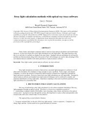
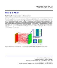
. . . . .APODIZ<strong>IN</strong>G BY ANGLES ON A VOLUME EMITTER US<strong>IN</strong>G ANEXTERNAL DATA FILEUSERAPOD ANGLES weights the angular flux of rays created by a table ofrelative intensity levels. The command is designed to work with goniometermeasurements. The syntax is shown below.Polar axisUSERAPOD ANGLES X ‘FILENAME’EMIT CONE X ... ISOThe ISOtropicoption is neededFile with relative intensity valuesIntensity of raysmirrors input pattern18 190 20 40 60 80 100 120 140 160 180 200 220 240 260 280 300 320 3400 0 0 0 0 0 0 0 0 0 0 0 0 0 0 0 0 0 010 10 10 10 10 10 10 10 10 10 10 10 10 10 10 10 0 0 020 30 30 30 30 30 30 30 30 30 30 30 30 30 30 30 0 0 030 90 90 90 90 90 90 90 90 90 90 90 90 90 90 90 0 0 040 95 95 95 95 95 95 95 95 95 95 95 95 95 95 95 5 5 550 82 82 82 82 82 82 82 82 82 82 82 82 82 82 82 2 2 260 75 75 75 75 75 75 75 75 75 75 75 75 75 75 75 5 5 570 71 71 71 71 71 71 71 71 71 71 71 71 71 71 71 1 1 180 70 70 70 70 70 70 70 70 70 70 70 70 70 70 70 0 0 090 70 70 70 70 70 70 70 70 70 70 70 70 70 70 70 0 0 0100 75 75 75 75 75 75 75 75 75 75 75 75 75 75 75 5 5 5110 70 70 70 70 70 70 70 70 70 70 70 70 70 70 70 0 0 0120 65 65 65 65 65 65 65 65 65 65 65 65 65 65 65 5 5 5130 65 65 65 65 65 65 65 65 65 65 65 65 65 65 65 5 5 5140 30 30 30 30 30 30 30 30 30 30 30 30 30 30 30 0 0 0150 15 15 15 15 15 15 15 15 15 15 15 15 15 15 15 5 5 5160 3 3 3 3 3 3 3 3 3 3 3 3 3 3 3 3 3 3170 0 0 0 0 0 0 0 0 0 0 0 0 0 0 0 0 0 0180 0 0 0 0 0 0 0 0 0 0 0 0 0 0 0 0 0 0RADIANT X; DISPLAY; MESH; $VIEW<strong>ASAP</strong> Technical Guide 21
. . . . .APODIZATION FILE FORMATNumber ofazimuthaldivisionsNumber of polardivisionsAzimuth angle(degrees)Low valuesduplicatedPolarangle(degrees)18 190 20 40 60 80 100 120 140 160 180 200 220 240 260 280 300 320 3400 0 0 0 0 0 0 0 0 0 0 0 0 0 0 0 0 0 010 10 10 10 10 10 10 10 10 10 10 10 10 10 10 10 0 0 020 30 30 30 30 30 30 30 30 30 30 30 30 30 30 30 0 0 030 90 90 90 90 90 90 90 90 90 90 90 90 90 90 90 0 0 040 95 95 95 95 95 95 95 95 95 95 95 95 95 95 95 5 5 550 82 82 82 82 82 82 82 82 82 82 82 82 82 82 82 2 2 260 75 75 75 75 75 75 75 75 75 75 75 75 75 75 75 5 5 570 71 71 71 71 71 71 71 71 71 71 71 71 71 71 71 1 1 180 70 70 70 70 70 70 70 70 70 70 70 70 70 70 70 0 0 090 70 70 70 70 70 70 70 70 70 70 70 70 70 70 70 0 0 0100 75 75 75 75 75 75 75 75 75 75 75 75 75 75 75 5 5 5110 70 70 70 70 70 70 70 70 70 70 70 70 70 70 70 0 0 0120 65 65 65 65 65 65 65 65 65 65 65 65 65 65 65 5 5 5130 65 65 65 65 65 65 65 65 65 65 65 65 65 65 65 5 5 5140 30 30 30 30 30 30 30 30 30 30 30 30 30 30 30 0 0 0150 15 15 15 15 15 15 15 15 15 15 15 15 15 15 15 5 5 5160 3 3 3 3 3 3 3 3 3 3 3 3 3 3 3 3 3 3170 0 0 0 0 0 0 0 0 0 0 0 0 0 0 0 0 0 0180 0 0 0 0 0 0 0 0 0 0 0 0 0 0 0 0 0 0Relative intensity values (candelas measured)NOTE: If the external file is formatted exactly as in the aboveexample, but given the filename, usap3d.n, where n is an integer,an alternative form of the command is given byUSERAPOD ANGLES X usap3d.nFunctions may also be used for apodizing a source. The default function is alwaysGaussian. To supply your own function, it must be defined in the usual way beforethe USERAPOD or APODIZE command is used. The general forms for apodizationwith a functional form are as follows:$FCN funct_name funct_definitionUSERAPOD POSITION [fcn] [c c’ c”...]USERAPOD DIRECTION [fcn] [c c’ c”...]<strong>ASAP</strong> Technical Guide 22
. . . . .NOTE: $FCN is a multipurpose <strong>ASAP</strong> macro, which can be calledfrom a variety of commands where a function is required. See theTechnical Guides, Predefined Macros and User-Defined Macrosfor more information on <strong>ASAP</strong> macros.If no data or function is specified, after calling for apodization with eitherUSERAPOD or APODIZE in this syntax, a Gaussian function is applied to thesource, by default. The form for the Gaussian isIn this case, c and c' are the semi-major widths of the Gaussian envelope. The c” isthe total flux in the beam. If a function is given, you can use up to 50 coefficientsto specify the functional form either in direction or positional space.When a function is provided, the function ($FCN) definition portion uses thevariables, _1 and _2 to represent the Cartesian coordinates or direction cosines. Inthe case of apodizing volume emitters in three-dimensional space, we can useUSERAPOD ANGLES with a function. In this case, the _1 and _2 variables are thepolar angle and azimuthal angle, respectively. An example script and output in the3D Viewer are shown below.RADIANT ZDISPLAYAVEMESH<strong>ASAP</strong> Technical Guide 23
A F<strong>IN</strong>AL NOTE ON APODIZATIONIf you want to apply more than one apodization to a source, do not use two or moreUSERAPOD commands in succession. <strong>ASAP</strong> uses only the last one defined.However, you may begin with a USERAPOD before the source is created, and usethe APODIZE command as many times as needed afterward.Immersing sourcesSources by default are defined to be in media 0, which is “vacuum/air”. If youneed to create a source in a different medium, such as in the LED example below,this needs to be told to <strong>ASAP</strong>, of course, or the ray trace will make incorrectrefraction calculations, and possibly generate wrong-side errors. This is thepurpose of the IMMERSE command. See the sidebar, “IMMERSE Command”.IMMERSE COMMANDIn many optical systems, the light source is not in air. The IMMERSE command causes all future rays to be created in thespecified medium until it is overridden by a new IMMERSE command. This is particularly useful in modeling LEDs.Example syntax:MEDIA; 1.49 ‘ACRYLLIC’IMMERSE ACRYLIC !! All future rays are created inside ACRYLIC (n=1.49)MEDIA; 1.5 ‘PLASTIC’Emit Rays insideIMMERSE PLASTICPLASTICENT OBJ; PLANE Z 1 RECT 2 2 ‘TOP’<strong>IN</strong>TERFACE COAT +BARE AIR PLASTICTUBE Z 1 2 2 0 2 2 1 1 ‘SIDES’<strong>IN</strong>TERFACE COAT +BARE AIR PLASTICPLANE Z 0.5 RECT 0.25 0.25 ‘DIE.TOP’TUBE Z 0.5 0.25 0.25 0.25 0.25 0.25 1 1 ‘DIE.SIDES’EMIT OBJECT 0.2 –50EMIT OBJECT 0.1 –25Emit rays from top and tides of diePLOT FACETS 1 1 OVERLAY; TRACE PLOT.24<strong>ASAP</strong> Technical Guide
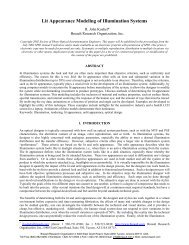
. . . . .Multiple wavelengthsWhen sources, coatings, or media are defined at different wavelengths, you mustspecify at the beginning of the file the range of wavelengths, including the onesyou are using, with the WAVELENGTHS command. Specify this range only once,as only the most recent WAVELENGTHS command detected by <strong>ASAP</strong> is the activeone.A limit exists for the number of wavelengths you may list (to determine your<strong>ASAP</strong> module limits, type DIMENSION in the Command Input window).Remember that the wavelengths must be listed in ascending or descending order.You can also specify this range, in connection with the SPECTRUM command. Ifyou use the list method, the MEDIA indices and COAT<strong>IN</strong>G PROPERTIES mustalso be listed in the same order, with one number or set of numbers given for eachwavelength. When the WAVELENGTHS command is used with the SPECTRUMcommand, up to 200 weights, along with the corresponding wavelengths from themost recent WAVELENGTHS command, can be used to create a multi-wavelengthspectrum of a source. See the SPECTRUM command in <strong>ASAP</strong> online Help.See Creating multi-color sources within <strong>ASAP</strong> with SPECTRUM on page 28.Here is a portion of an example of creating multiple sources at differentwavelengths:Example: Creating multiple sources at different wavelengths (portion of script)NOTE: Rays have only a single wavelength associated with them.When each source is created later in the file, a wavelength isassigned for that set of rays, using the WAVELENGTH command.<strong>ASAP</strong> performs a linear interpolation for any source wavelengthsbetween those stated at the top of the file. For this reason, do not<strong>ASAP</strong> Technical Guide 25
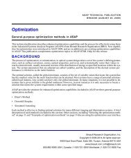
use wavelengths falling outside the WAVELENGTHS range, orcalculations may be unreliable. The script shown in “A simple lenswith a built-in glass catalog” on page 27 produced the plot, “Twodimensionalgrid sources”.Two-dimensional grid sourcesWe constructed a simple lens and used the built-in glass catalog for SCHOTT BK7glass, rather than specifying our own indices, as in the above example. Threeseparate, two-dimensional grid sources were made at red, blue, and greenwavelengths in identical positions and sent through the lens. You can see thedispersion that resulted from the difference in refractive indices at the threewavelengths.Notice that we used the technique of tracing the sources individually to control thecolor of the corresponding wavelengths. As long as each source has a wavelengththat is different from the other sources, the TRACE command can be run with allthe sources at the same time, and produce essentially the same result as the aboveplot.26<strong>ASAP</strong> Technical Guide
. . . . .A simple lens with a built-in glass catalog<strong>ASAP</strong> Technical Guide 27
Creating multi-color sources within <strong>ASAP</strong> with SPECTRUMSources in <strong>ASAP</strong> are usually created at a single wavelength that is defined by themost recent WAVELENGTH command. Multiple color sources are created bydefining rays at separate wavelengths. The SPECTRUM command is used toweight the flux of rays according to a user-defined spectral power distribution or atable of weights, shown below.PHOTOPICStandard Luminosity Curve (Eye response in bright light)SCOTOPICStandard Luminosity Curve (Eye response in dim light)THERMAL Power output of a blackbody at temperature T (degrees K)PHOTONS Photons/second of a blackbody at temperature T (degrees K)w w’ w” w’”... Table of weightsThis technical guide discusses thermal (blackbody sources) and numericalwavelength weighting of multi-color sources. For a discussion of the standard eyeresponse curves, see “CIE numerical and graphical color analysis” in the <strong>ASAP</strong>technical guide, Radiometric Analysis.BLACKBODY RADIATORS - THERMALThe SPECTRUM THERMAL command gives <strong>ASAP</strong> the ability to simulate thethermal emission of an object at a given temperature. This type of source can beused as a blackbody radiator. The spectral power of a blackbody emitter is shownbelow along with the <strong>ASAP</strong> script used to produce the plot.Example: Spectral power of a blackbody emitter28<strong>ASAP</strong> Technical Guide
. . . . .Example: Blackbody emitterThe function that calculates the source total flux requires integrating over a rangeof wavelengths. Since <strong>ASAP</strong> normally allows only a single wavelength to beassigned to a source, the flux must be modified by a separate calculation after thesource is created. The initial source must be a Lambertian emitter. Therefore, it iseither an emitting surface or an emitting object.A formula, based on the Stefan-Boltzmann law, is then applied using an arithmeticoperator in <strong>ASAP</strong>. This is called the “FBI” (Fractional Blackbody Integral)function. The following parameters are needed for the formula:• Surface area of the emitter,• Wavelength interval to integrate over,• Temperature of the radiator in degrees-Kelvin, and• Emissivity of the source (from 0 to 1, where 1 would be a perfect blackbodyradiator and 0 would be non-radiating).<strong>ASAP</strong> Technical Guide 29
The function integrates over the specified spectral range or interval. The result isthe radiant emittance in Watts/cm2. If the interval is equal to the unit in which thewavelengths are measured (such as 1 micron), the result is the spectral radiantemittance in Watts/cm2/(wavelength unit). If the surface of a cube is, for example,a blackbody radiator in the infrared, you can set up the source and assign its fluxsimilar to “Example: Setting up the source for a black body radiator in theinfrared”.Example: Setting up the source for a black body radiator in the infraredThe variable POWER represents the critical expression, which gives us the radiantemittance of the blackbody source. We simply apply that to the flux total after thesource is created. Since we want the flux to be in Watts, we changed the nameusing the UNITS command.BLACKBODY RADIATORS - PHOTONSThe same script used in “Example: Setting up the source for a black body radiatorin the infrared” can be used to produce a spectrum of photons/sec emitted by ablackbody emitter by usingSPECTRUM PHOTONS (temperature)The result is shown below.30<strong>ASAP</strong> Technical Guide
. . . . .Spectrum of photons/sec emitted by a blackbody emitterSPECTRAL APODIZATION WITH A TABLE OF WEIGHTSIn “Spectrum of photons/sec emitted by a blackbody emitter”, a table of weights isused to apodize the source spectrally. Up to 200 weights, along with thecorresponding wavelengths from the most recent WAVELENGTHS command, canbe used to create a multi-wavelength spectrum. The result of this apodization andthe <strong>ASAP</strong> script that produced this result is shown in “Example: Spectralapodization with a table of weights and script”.<strong>ASAP</strong> Technical Guide 31
Example: Spectral apodization with a table of weights and script32<strong>ASAP</strong> Technical Guide
. . . . .Setting the fluxAs discussed in Chapter 8 of the <strong>ASAP</strong> Primer, the FLUX command allows severalmethods for setting the total flux or normalizing the flux of a source to some value,which might be based on a previous flux calculation. The FLUX commandoperates on all currently selected rays. This means you can select the rays youwant to modify using the SELECT ONLY command. If there are multiple sources,the FLUX command by itself affects all the sources that are created, unless statedexplicitly in the Command Input window, or by using SELECT ONLY with asource (relative or absolute reference) number. Take the following case whereseveral grid sources are created and each needs a specific level of flux assigned:If we do not use SOURCE 0.1 as a relative referencing to the previous sourcedefined, each FLUX TOTAL command applies to all the sources taken together,thereby overriding previous definitions. The following script accomplishes thesame thing, but at a different point in the file.FLUX TOTAL distributes the total flux among the sources in proportion to thevalue each source has before the command is applied. In the following case, threedifferent sources are created. Remember that emitting sources have unit flux, whilegrid sources have unit irradiance.<strong>ASAP</strong> Technical Guide 33
In this case, the first source has (4/21)*100 units, the second source has(16/21)*100 units, and the third source has (1/21)*100 units. We could also assignflux to each source individually in the following manner:Finally, <strong>ASAP</strong> can adjust the flux of each currently selected and considered raywith the command:FLUX a bThe meaning of this flux adjustment for each individual ray is given by thefollowing expression:We mentioned earlier, and it is worth repeating here, that <strong>ASAP</strong> uses “flux” as adefault name for the energy of the rays or beams. This name can be changed to anyname desired, such as “lumens”, “candela”, or “Watts”. It is assigned through theUNITS command as the optional second argument:UNITS length ‘flux_name’ReviewAs you can see now, sources come in a variety of forms. Aside from all the built-intypes, external files can also be imported. The BRO Light Source Library isaccessed via menu commands, while $READ can directly import ray files. <strong>ASAP</strong>sources can be obtained from Radiant Imaging, <strong>Inc</strong>. Objects can be imported fromCAD programs and made into emitting surface objects.We learned that flux levels can be initialized to any value and modified at any timelater, if desired, using the FLUX command. The unit name can also be changedwith the UNITS command to make it clearer for plots and statistical data.34<strong>ASAP</strong> Technical Guide
. . . . .An isotropic source can be modified to match real-world measurements byapplying spatial, directional, or angular apodization. This is done with either theUSERAPOD or APODIZE commands. For applications such as LEDs, we foundthat the IMMERSE command is necessary to force the source to begin in a mediumother than vacuum/air.We also know the basic rule of one wavelength per source. However, if we havemultiple wavelength-dependent coatings, indices, or sources, we must specify awavelength range that covers them all. This specification is done once at the top ofthe file.With the SPECTRUM command, <strong>ASAP</strong> can produce standard eye response curves,blackbody spectra, and spectra weighted with user-supplied weights, whichcorrespond to a series of wavelengths specified with the WAVELENGTHScommand.<strong>ASAP</strong> Technical Guide 35